Description and justification

1 Experimental set-up

Fibrillating hearts of 17 dogs (Beagles) were studied during complete cardiopulmonary bypass and coronary perfusion. In a fibrillating heart without coronary perfusion the fibrillation changes progressively, whereas in a perfused heart the fibrillation may be stable for very long periods (Hoffman 1960). No effect has been found of ventricular fibrillation on the function of the heart when the normal circulation and nourishment of the myocardium was maintained (Surawicz 1971). Except for the experiments described in chapter XI these dogs were not especially meant for this study, but belonged to the control groups of other experiments. The procedure to keep a dog on total cardiopulmonary bypass while maintaining a good general condition has been described in detail by Runne 1976, de Vries 1976 and Stokhof 1976 This procedure can be summarized as follows.

1. The dogs did not receive premedication.
2. Anesthesia was induced with 25 mg thiopental per kg body weight intravenously and maintained by adding halothane to the gas mixture (97.5% oxygen and 2.5% carbon dioxide) of the bubble gas oxygenator (Bently Q110). The blood was circulated by a roller pump (Sarns 2000), controlled by an automatic feed-back system that maintained either a constant (mean) pressure in the aorta or a fixed flow through the arterial line or a constant amount of blood in the oxygenator. In one experiment these three modes have been compared; all other experiments were done in the constant aortic pressure mode of 70 mm Hg.
3. An arterial line temperature of 38°C was maintained.

In order to form a link between the results obtained in the group of healthy, perfused dogs and the results in the group of coronary care patients, in two healthy, anesthetized dogs ventricular fibrillation was induced without artificial coronary perfusion.

In all cases, except the experiment described in chapter 11 (par. 5) ventricular fibrillation was induced by stimulating the heart by a 24 V 50 Hz current during several seconds. The heart of the dog used for that experiment was stimulated via a programmable stimulator (van Poelgeest 1976 and van Laar 1985).

2 Patient data

Spontaneous ventricular fibrillation in coronary care patients of the St. Antonius Hospital, Nieuwegein, could be analyzed when the ECG of one of the standard leads had been recorded on magnetic tape during fibrillation. In one case ventricular fibrillation could be studied in a 60 year old man without clinical symptoms of myocardial infarction, who accidentally got fibrillation during the introduction of a catheter in the right ventricle. (University Hospital Utrecht).

3 Electrodes, leads and amplifiers

The following types of electrodes were used:

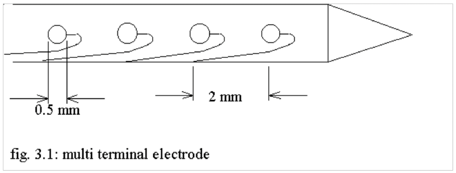
1. a multi-electrode needle carrying 20 platinum terminals, of 0.25 mm diameter each, interterminal distance being 2 mm (Durrer 1964) was introduced into the septum perpendicular to the epicardium;

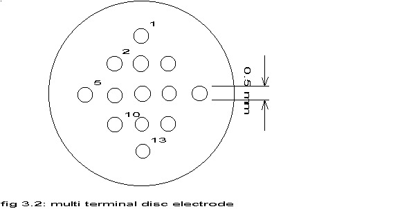
2. a multi-terminal disc carrying 13 platinum terminals, of 0.25 mm diameter each, interterminal distance being 1 mm, arranged according to the pattern shown in the figure above; this disc was attached to the epicardium.

3. abbreviations

A	Aorta
Ap	Arteria pulmonalis
La	Left atrium
Lv	Left ventricle
Ra	Right atrium
Rv	Right ventricle
Vci	Vena cava inferior
Vcs	Vena cava superior

4. single epicardial electrodes, primarily used to record atrial activity during ventricular fibrillation; standard arrangement of the epicardial electrodes is shown in figure 3.3.
5. standard leads.

Bipolar leads between adjacent terminals and/or unipolar leads between a terminal and a needle inserted subcutaneously into the left hindleg and/or ECG lead II were stored on analog tape by FM techniques via normal ECG amplifiers with a frequency band of 0.5 Hz to 5000 Hz. Long term (> 2 hours) recording of unipolar leads was hampered however by polarization of the terminals, so the department of medical physics developed an amplifier based upon an optically coupled linear isolation amplifier (Burr-Brown 3652) to avoid this problem.
The term electrogram or cardiac electrogram will be used for the recordings from electrodes directly upon or in the heart tissue, in contrast to the ECG, recorded from the surface of the body (Hoffman 1960 and WHO 1978). According to Hoffman and Cranefield the unipolar electrogram is most useful to study the direction and velocity of the spread of activation. The “intrinsic deflection” coincides with the depolarization of cells near to the electrode. Injuries however will lead to so-called local injury potentials. Intramural needle electrodes cause minimal damage to the myocardial tissue and no local injury potentials have been found (Spach 1975). The bipolar electrogram is most useful to determine activation time in a large body of tissue. The velocity and direction of the wavefront has a strong influence upon the amplitude and shape of the recorded potentials (Hoffman 1960). Most of the work in this investigation was done with unipolar leads. Theoretical and practical difficulties in calibrating the potentials measured by the electrodes, led to the decision to record all signals uncalibrated. See also table 3 in chapter VII.

4 Signal analysis

In this paragraph the general classification by Zetterberg (Zetterberg 1977) of the means and methods for digital processing of physiological signals will be followed.

4.1 Objectives

The electrograms mentioned above represent a large body of data. Consequently, signal processing in general aims at data reduction and information extraction. The main objectives are:

1. Elimination of disturbances and reduction of data without loss of relevant information. The available recordings were screened to select appropriate parts for further analysis, which of course introduces a subjective element. Filtering was performed prior to conversion to digital data in order to remove undesirable, high frequencies (par. 4.3: Signal categories), but not for noise reduction, as the distinction between relevant data and noise was not known a priori.
2. Description of characteristic properties of ventricular fibrillation. The aim is in general the calculation of a limited number of essential descriptors. The major aim of this study is to find such descriptors.
3. Relationships between characteristic properties of ventricular fibrillation and physiological variables. Some modest attempts are described in chapter XI.
4. Decision in order to distinguish between hypotheses and to carry out diagnosis in combination with other information. No attempt has been made to fulfil this objective.

4.2 Information aspects

The objectives reflect the amount of information that is available about a physiological process. As far as a priori information is concerned, the following three situations may be identified:

1. The exploratory phase with a very limited amount of signal analytical knowledge available, in which this study started. The exploration is described in chapter IV and chapter VII;
2. The interesting characteristics of ventricular fibrillation may be defined, as is done in chapter VI and chapter IX;
3. Sufficient information is available to formulate mathematical models, see chapters V, VIII and XII.

4.3 Signal categories

To proceed the type of signal to be analyzed has to be defined. From a functional point of view the following three types may be distinguished:

1. Point processes. These describe time discrete events like heart beats. Although a lot of work in the field of ventricular fibrillation has been done by comparing activation times with the help of intrinsic deflections (Hoffman 1960) no objective criteria could be found to detect these deflections in the recordings from the dogs, in accordance with the general remark of Surawicz (1971) and the special remark of Janse (1980) upon unipolar recordings from the dog heart. Zero crossings may also be considered as significant events in the signal to be analyzed. A problem will be to identify both the presence of low and high frequency waves. Moreover, preliminary checks on multichannel recordings of electrograms during ventricular fibrillation showed vast differences in numbers of zero crossings in neighbouring electrodes, so this method was considered impractical and inadequate for this study. Both problems could be caused by excitations traversing the myocardium parallel to the muscle fibers and perpendicular to them at the same time, as in that case largely different intrinsic deflections will be recorded (Corbin 1977)
2. Spontaneous activity giving rise to time-continuous signals, like all signals analyzed in this study.
3. Stimulated functional activity like the study of conduction in the heart by programmed stimulation, etc. One experiment has been performed (chapter XI)

From a technical point of view the next four types of signals may be distinguished.

1. Transient signals, i.e. signals that have a short duration compared to observation time. This type has not been encountered in ventricular fibrillation.
2. Periodic signals; according to the theories mentioned in chapter II, ventricular fibrillation was at the start of this study not considered to be periodic.
3. Stationary stochastic signals; a mathematical idealization, which says that certain properties – like mean value, autocovariance, probability distribution function – are invariant to a shift in time. The electrical signals recorded during ventricular fibrillation in dogs with artificial coronary perfusion were assumed to belong to this class of signals.
4. Nonstationary stochastic signals; a vast number of possibilities. Interest is restricted to systems with time variable parameters that either change slowly with time compared to the process itself – like ventricular fibrillation without artificial coronary perfusion – or change suddenly in jumps, but so infrequently that the system in between may be considered to have fixed parameters – like the rather sudden jump from sinus rhythm or ventricular tachycardia to ventricular fibrillation.

4.4 signal processing methods

Compare with fig. 4.1

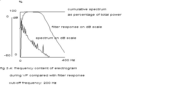
Although in principle signal analysis with e.g. analog filters is possible, only digital methods have been considered. The recorded analog signals were converted to digital values by the PDP-15 computer of the cardiology department. Prior to conversion the signals were passed through a bandpass filter plus amplifier set (Difa FB06/AB100) – highpass filter 0.01 Hz and lowpass 6-pole Butterworth filter with a response of 36 dB per octave from the cut-off frequency. See fig. 3.4 with a cut-off frequency of 200 Hz.

This subparagraph will describe in general terms which methods were tried and were considered success or failure. The failures are indicated in this paragraph, the successes in the next chapters. The exact formulas used and their justification will be found in the appendices in chapter XIV. The essential distinction has to be made between parametric and nonparametric methods. The first are tailored to fit a specific model of the process, determined by a set of parameters. Fitting an autoregressive and/or moving average model (Box and enkins 1970) to a sequence of data may serve as an example. Preliminary checks of the usefulness of the Box and Jenkins approach to describe the fibrillation signals, revealed that none of the tried signals could be described by autoregressive models, indicating a strong non-linearity in the signals, which formed the first clue for the development of the model of chapter V. Modern methods of frequency analysis depend in some way or other on autoregressive descriptions, (e.g. Linkens 1978, Linkens 1979f and Schlatter 1979) so they too were considered inadequate.

The nonparametric methods are applicable to a variety of signals and do not require specific assumptions about the processes in terms of models. Fourier analysis, correlation analysis and more general descriptions like amplitude histograms are examples of these methods. The first analyzed signals did not contain appreciable power in frequencies above 40 Hz (fig. 3.4), so a standard sampling frequency for A/D conversion of 100 Hz, a cut-off frequency of 30 Hz and a duration of 40 sec’s were chosen. This implies that the -40 dB point is reached at 64.5 Hz, so – because of aliasing – the analysis of frequencies above 35.5 Hz should be taken with a pinch of salt.

The converted values were stored on digital tape (Herbschleb 1976) and in majority analyzed on the Cyber 175 computer of the computer centre of the University of Utrecht by the frequency analysis programs especially developed for this study (thanks to grant 74.101 of the Netherlands Heart Foundation, Jan Klein Douwel and Ingeborg van der Tweel) and partly by a similar package on the PDP-15 computer of the Cardiology department. Considerations of computing efficiency, memory usage and digital storage facilities lead to division of the digitized signals into 20 consecutive blocks with a length of 2 sec’s. From each block its mean was subtracted. Next, the blocks were doubled in length by adding zeroes and using standard FFT routines the Fourier transforms of these blocks were computed and stored on digital tape. See appendix A.

Another distinction often made is between methods that operate primarily in the frequency domain and those that operate in the time domain. This distinction is not an essential one, as both methods describe the same phenomenon in two different ways, but a practical one, as some researchers are more at home in the time domain and others in the frequency domain. In the frequency domain were estimated from the Fourier transforms the auto power spectra (chapters IV, X, XIand appendix A), autobicoherency spectra (chapters IV, X, XI and appendix D), cross phase spectra (chapter VII and appendix C). and squared coherency spectra (chapters (VII and XI and appendix C).

In the time domain amplitude histograms were constructed directly from the digitized signals in order to determine the probability distribution of the electrogram amplitudes. The histograms were classified as symmetrical, skewed, uniform or bipolar. To facilitate this classification the curve was plotted of the best fitting Normal distribution, i.e. with the same mean and standard deviation as the histogram. If the histogram looked symmetrical a Kolmogorov-Smirnov test was applied in order to see whether the amplitudes fitted a Normal distribution or not. From the Fourier transforms the autocorrelation functions (chapters IV, X and XI and appendix B) were estimated.

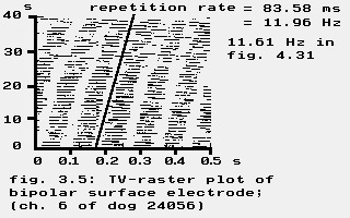
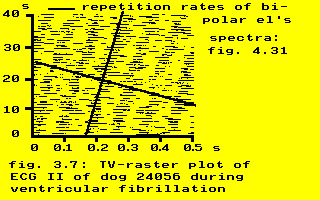
A rather simple way to find a repetitive pattern in signals is to plot the signal in the TV-raster format as used in circadian research (Winfree 1982c): the time axis is broken up into consecutive equal intervals stacked from bottom to top, with black lines representing positive values.

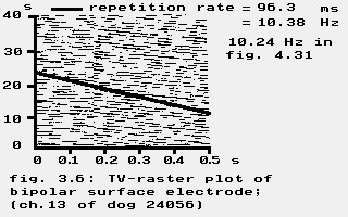
See the autopowerspectrum in fig. 4.31. Compare with fig. 4.19.

Figures 3.5 and 3.7 clearly indicate a repetitive pattern during ventricular fibrillation, contrary to figure 3.6. Frequency analysis however fig. 4.27 shows a clear peak, indicating a rather regular repetition rate. Rapid changes in the shape of regularly repeated electrical complexes will distort the TV-raster plots much more than the power spectrum; a similar observation was already made by Rothberger and Winterberg in 1916 (Rothberger 1916). A slow change in shape will give an impression of regular repetition, but in that case the repetition rate measured in the TV-raster plot will slightly differ from the repetition frequency in the power spectrum (11.96 Hz according to figures 3.5 and 3.7 versus 11.61 Hz in figure 4.31).
Conclusion: TV-raster plots are nice illustrations, but cannot be used for signal analysis.

A mixture between time and frequency domain will be found in chapter X, where the dynamics of the auto power spectrum is described.