VIII. WEAKLY COUPLED RELAXATION OSCILLATORS AS A HIGHER LEVEL MODEL OF VENTRICULAR FIBRILLATION

1 Introduction

A model of the whole heart at the cellular level is impossible because of the immense number of cellular connections. Immense is used in the sense of Elsasser (see Scott 1977 ). So a higher level model is required and by describing the ventricles during ventricular fibrillation as a system of weakly coupled relaxation oscillators, a reduction in the number of elements of at least 1000 is achieved. The relaxation oscillators meant are described in chapter V, par. 3 as a patch of 1000 cells, dimensioned 1 * 0.1 * 0.1 mm, in persistent activity and displaying the ability to get synchronized or entrained by external stimuli. These relaxation oscillators are considered weakly coupled as at most 100 of the 1000 cells border another relaxation oscillator. The total number of relaxation oscillators needed to model the whole ventricle is nevertheless still very large. A further reduction is of course possible by enlarging the size of the relaxation oscillator. The number of 1000 cells was chosen for practical, computational reasons, but the overall dimensions cannot be more than 1 mm (see chapterVII, par. 3 . Even then the model of the ventricle would consist of a hundredthousand relaxation oscillators coupled in a three-dimensional network. Such a big number requires analytical approaches like a field theory for networks of excitable elements or catastrophe theory for Van der Pol oscillators, e.g. Zabara 1971 , Guettinger 1974 or Joyner 1975 , or maybe extensive analysis of the behaviour of the chemical Turing system, e.g. Hermens 1972 or Winfree 1980 , but at the moment we can still agree with: “the analysis of complex networks of excitable networks is generally refractory to analytical approaches” (Rosen 1977 ).

Much more modestly this chapter will explain the rather local phenomena described in chapter VII in terms of relatively small numbers of coupled relaxation oscillators and indicate the consequences of viewing the whole fibrillating ventricle as a mass of relaxation oscillators.

No confusion should arise with the models of coupled relaxation oscillators to describe normal heart beating. Pioneering work was already done in the 1920’s (van der Pol 1929 ). In these models the ventricle is seen as one relaxation oscillator coupled to another one representing the atrio-ventricular node ( Power 1979 ); no ventricular fibrillation is possible in Power’s model and he states about ventricular fibrillation: “..it seems likely that they (the high frequencies) reflect the chaotic, zigzag pattern of wave travel in that arrhythmia rather than the maximum firing rate of individual cells” . His model does not allow ventricular fibrillation, but extending the widely known function of Van der Pol with a third power of x by suitable scaled fifth and seventh powers, creates a relaxation oscillator with two strongly different rhythms. Transitions from normal beating to ventricular fibrillation can thus be simulated, but as the physiological implications of this model are not clear, no further attention will be paid to it in this study.

2 A cellular oscillator

2.1 Introduction

In the preceding paragraphs ventricular fibrillation has been described as a phenomenon based upon the concept of individual myocardial cells being more or less synchronously, but very regularly active. Both the spectral analysis and data from literature indicate that the apparently very high repetition frequency during ventricular fibrillation is caused by two almost equal groups of synchronized cells beating at half the fibrillation frequency, with half a period delay between these groups. In order to get more insight in the mechanism required for such a behaviour a model for the local fibrillation has been developed, consisting of 1000 interconnected cells in a threedimensional structure. The fact that this model behaved as a relaxation oscillator has been used as justification to describe the large scale phenomena during ventricular fibrillation as stemming from a network of connected relaxation oscillators. A lot of unanswered questions arise from both the physiological assumptions and the mathematical model, which will require much more experimental and mathematical effort to get some answers.

2.2 Uniform phase distribution at start of fibrillation

The model of local fibrillation of chapter V starts with all cells uniformly distributed over the possible phases. This means that at every timestep the same number of cells became active. Nevertheless, at certain parameter settings, after an initial period the spontaneous activity showed peaks in the course of time; the period between these peaks was half the repetition period of the individual cells. Although it is not known whether such a distribution of phases is possible in reality or not (but see chapter VI, par. 4.2 ), if we assume its possibility and a small variability in the total refractory period between neighbouring cells, then very rapid pacing of the myocardium will after some time bring all cells in a different phase. If all cells are in a different phase, then ventricular fibrillation is inevitable according to the model and the period of rapid stimulation required to start ventricular fibrillation can be used to estimate the upper limit of variability amongst cells.

In the experiment described in chapter XI, par. 5 a stimulation period of 10 seconds was required in order to start fibrillation. During stimulation at 50 Hz the heart was beating at 8.25 Hz (= 121.2 ms R-R interval or 495 b.p.m.) and after 82.5 beats a completely uniform distribution would have been reached if the total range of variability in the refractory period amounted to 1/82.5 cycle, i.e. 1.4 ms with a median of 121.2 ms. Of course this result only indicates the order of magnitude and these assumptions should be tested much more thoroughly.

2.3 Local fibrillation model – two cells

The model in chapter V, par. 3 required a large computer and a lot of computation time for each new parameter setting; although now a PC-version is available (see topolt . Another drawback is the fact that the model is not suitable for further mathematical research. An attempt will be made in this chapter to provide a set of smooth differential equations that describe the behaviour of the model and lends itself to a more extensive analysis. In the model, cells could have a lot of nexuses in common or just a few. The attention will be focussed on two strongly connected cells and the input on all other nexuses will be considered as background noise.

Implicit in the model are jump functions, i.e. a cell is active or not, absolute refractory or not, etc. As these functions cannot be differentiated over the whole range, they are approximated in this paragraph by arctan functions:

1. S(x) = 0.5 + arctan(px) / π
   The larger the factor p, the better this function resembles a jump from 0 to 1 at x=0.

In order to study the influence of two strongly connected cells with a certain phase difference on each other the cells have been made oscillators by setting the background activity higher than the threshold.
The following notation will be used: N total number of nexuses per cell Nt threshold in number of nexuses Na Number of nexuses between 2 strongly connected cells Nb background activity in number of active nexuses Te length of excited period Ta length of active period Tr length of absolute refractory period F accomodation factor

The threshold function in the relative refractory period has been defined in chapter V as:

1. g( ) = exp(0.22( ·T – Ta – Tr – 21)
   where T stands for the repetition period if only background activity is present and is calculated as:
2. T = 21 / (1 – F·Nb/N) + Te + Ta + Tr
   The phase is defined as the time spent in a certain period divided by T, runs thus from 0 to 1 and is set at 0 at the start of activation (not excitation).
   The number of active nexuses of a cell is determined by the background activity and by the fact whether the strongly connected cell is active or not, and is denoted by:
3. Nact( ) = Nb + Na·S(Ta/T)
   The passing of the threshold by the total activity is governed by the function:
4. f(Nf) = S(Nt + g( ) – Nact( ))
   With these functions now an expression for the rate of change of can be given:
5. 1 : phase of cell 1
   2 : phase of cell 2
   d 1/dt = (1-S( 1-(Ta+Tr)/T)·(S(Ta/T- 2)· (((1- 1)·T/Te-1)·f(-N 2) – F·Nact( 2)/N·f(N 2)))/T

The following situations are to be considered:

1. The first S-function is 0 if cell 1 is active or absolute refractory and the second S-function is 0 if cell 2 is not active, meaning that in those cases the phase of cell 1 follows its course undisturbed.
2. If cell 1 is relative refractory and cell 2 is active, two outcomes are possible.
   1. If the threshold is passed by the total activity then d 1/dt=(1- 1)/Te, which simply means that the cell becomes active after Te, keeping in mind has been defined modulo 1.
   2. If the threshold is not reached accomodation occurs as d 1/dt=(1-F·Nact( 2)/N)/T will be lower than 1/T. This may lead to delay.

The behaviour of the second cell is of course also given by [eq. 6] with the suffixes 1 and 2 interchanged. This set of differential equations can be used to study the change in phase relation and/or periodicity of two strongly connected cells like the cells in the model of chapter V, par. 3 .

For some parameter settings this behaviour has been checked for ‘s of 0, 0.1, 0.2, 0.3, 0.4, 0.5, 0.6, 0.7, 0.8 and 0.9. The results are summarized in the next table.

Nb	T	period decrease as % of T					of accelerated pairs
		Nt =					Ta = 95								85						75				65				55
		1	10	15	25	32	Tr = 5								15						25				35				45
50	145.2	74	76	77	79	81	0	0.1	0.2~	0.4~	0.5	0.6	0.7		0	0.1`	0.5`	0.6	0.7		0	0.6	0.7		0~	0.6~	0.7
40	136.7	80	81	82	84	86	0	0.1	0.2~	0.4~	0.5	0.6	0.7		0	0.1`	0.5`	0.6	0.7		0	0.6	0.7				0.7		0.7
30	130.9″	83	84	85	88		0	0.1	0.2~	0.4~	0.5	0.6	0.7	0.8	0	0.1`	0.5`	0.6	0.7	0.8	0′	0.6′	0.7	0.8			0.7
20	126.7	86	88	89			0	0.1			0.5	0.6	0.7	0.8	0	0.1~	0.5~	0.6	0.7	0.8	0	0.6	0.7	0.8			0.7	0.8
10	123.5	89					0	0.1			0.5	0.6	0.7	0.8	0	0.1	0.5	0.6	0.7	0.8	0	0.6	0.7	0.8			0.7	0.8
2	121.5	92					0	0.1			0.5	0.6	0.7	0.8	0	0.1			0.7	0.8	0	0.6	0.7	0.8			0.7	0.8
~ : Nt=1; `: Nt<25; ‘: Nt<32

The most striking result is that the synchronized cells run with the same period as cells with only background activity, but the cells that do not affect each others phase run much faster.
In the next table these shorter periods are compared to the model studies of chapter V .

1000 cell model of chapter V				repetition period of
threshold	average nr	period of central cell		strongly connected cells
	of active	in timesteps		in antiphase
	nexuses	mean	SD	formula 10
1	40	107.8	0.44	107.77
15	50	111.5	0.67	111.46
25	42	114.0	1.13	113.80

The fact that the periods calculated with the help of eq. 10 agree with those from the models, indicates that the behaviour of the model of 1000 cells strongly depends upon the mutual influence of two strongly connected cells.

For the most extensively studied model in chapter V, par. 3.3 with Te=3, Ta=85, Tr=12, N=70, Na=18, F=0.75 and an average activity of circa 710 cells (so Nb=50) the behaviour of [8.6] has been calculated for 1 and 2 ranging from 0 to 0.99 with increments of 0.01 (Te, Ta and Tr in model timesteps). The results are sketched in the following figure, where S indicates the area with equal phase and low periodicity, and where A indicates the areas with unchanged phases and high periodicity. The arrows indicate areas where the phase differences shift to the area indicated by the accompanying character. In figure 8.1 the phases are expressed as fraction of the background period, but as the cells in area A run 1.3 times faster their phases have been recalculated as fraction of this new period. The middle of the areas A then fits a phase difference of 0.5 between the two cells.

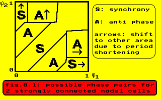
The fast cells have a period of 112 steps in this case, although the shortest possible period would have been 103, which is connected with the border between A and A-arrow in this figure. The models, experiments and literature cited point to the same phenomenon.

2.4 Local fibrillation – two groups of cells

The result of the preceding paragraph is valid for all strongly connected cells in the aggregate of 1000 cells. The cells with equal phase do not really influence each others period, whereas the cells with a stable phase difference stimulate each other to a higher repetition frequency. This means that the phase difference between a fast and a slow cell is not constant, in other words if the phase difference lies in area A of fig. 8.1 the slow cell is speeded up and if the phase difference lies in area S then after a few cycles the phase difference enters an A area and the slower cell is also speeded up. Two strongly connected cells can be speeded up by their respective neighbours and have the same phase, as they do not influence each others frequency in that case. The consequence of this reasoning is that in an aggregate of strongly connected cells the only stable modes are anti-phase and in-phase, as all other phase differences will lead at some distance in time to unstable differences. The model of chapter V is more complicated, because also weak connections are present, but the result of eq. 6 remains the same if one cell with strong connections is replaced by several synchronous cells with weak connections.

If the reasoning is accepted that – at least in the model – during ventricular fibrillation every cell is connected to a cell in antiphase, the new frequency of the aggregate can be calculated as follows. The phase where a cell passes the threshold follows from eq. 2 and eq. 3:

1. t = (Ta + Tr + 21 – ln(Nb + Na – Nt)/0.22)/T
   The rate of change of the phase in the relative refractory period follows from eq. 4 and eq. 6:
2. /dt = (1 – F·(Nb + Na)/N)/T
   The time spent in this period now clearly is:
3. = ( t – (Ta + Tr)/T)/(d /dt)
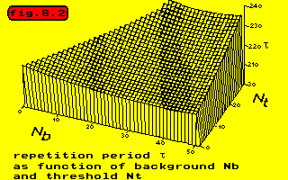
   and the new period will be:
4. = Te + Ta + Tr +

In the next figure the repetition period has been sketched as a function of the background activity and the threshold.

Once the cells in an aggregate have organized themselves into two groups in antiphase, the behaviour of the aggregate can be described in a simple way.

The notations of the preceding subparagraph have been augmented: N total number of nexuses per cell Nt threshold in number of nexuses Na Number of nexuses between 2 strongly connected cells Nb background activity in number of active nexuses NE number of active nexuses from environment Ni average number of nexuses for connection type i Mi number of cells of type i connected to one cell I number of types of connections Te length of excited period Ta length of active period Tr length of absolute refractory period F accomodation factor p(t) fraction newly active cells in an aggregate of cells

One group of cells is activating the other and after half a period vice versa. The maximal fraction of cells that can become active at a certain time is equal to 1 minus the fraction active cells. The chance of becoming active is equal to 1 minus the chance that the number of active nexuses is lower than the threshold.

This leads to the formula:

11. p(t+1) = (1 – p(t))·(1 – P0)

P0, the probability that the sum of active nexuses is lower than the threshold, can be calculated exactly, using a tabulated density function, but in this study a binomial approximation is used. P0 is thus the probability that not enough neighbours are active, using the average number of nexuses per neighbour.

Afbeelding van formule ontbreekt.

The behaviour of the complicated model of chapter 5 has now been idealized to a nonlinear difference equation 11, where the length of the discrete steps is /2 eq. 10.

2.5 A computer model

Based upon the formulas 1 through 12 a program ( vfsum ) has been made that shows the behaviour of the oscillator. The parameters of the program have the same values as the parameters of topolt of chapter V.

3 Synchrony, entrainment or chaos

Some of the regular amplitude variations in electrograms during ventricular fibrillation can be ascribed to amplitude pulsation, caused by the summation at the electrode of two or more signals with slightly different fundamental frequencies. Other variations however looked like true amplitude modulations and the variations were too regular to be ascribed to stochastic variations in the fundamental frequency (chapter IV, par. 8 and appendix E ). The modulations will be explained with the theory of coupled relaxation oscillators together with the shifts of coherent areas and the slow phase shifts between almost entrained areas chapter VII, par. 3 . The definitions of Winfree are kept: by entrainment is meant a locking together of frequencies, though not necessarily with a stable phase relationship; by synchrony is meant entrainment with, in addition, exact lock-step of phase. Winfree 1980 . A lot of work has been done on relaxation oscillators coupled via a common medium, in Winfree (1980) a long list of references will be found, but much less on mutually coupled relaxation oscillators, specially analytical work.

The amplitude pulsation and modulation phenomena can be explained by the theoretical work of Linkens Linkens 1979a , Linkens 1979b , Linkens 1979c , Linkens 1979d and Linkens 1979e . Very weakly coupled relaxation oscillators display beatings in the overall, externally measured behaviour, like shown for the ECG in fig. 4.30 . The ECG can be considered as a weighted sum of all signals arising from the heart and widely spaced oscillators are independent chapter VII, par. 3 or at the most very weakly coupled. The variations however of the electrograms from epicardial or intramural electrodes cannot be explained as amplitude pulsation, as no clear double peaks have been found after “zooming in” on the fundamental frequency peak. One electrogram expresses the electrical activity of a tiny area of the heart and if there is more than one oscillator in that area, a moderate coupling should be assumed. Linkens shows how in this case modulation arises, both in frequency and amplitude. Both types of modulation give rise to symmetrical sidebands, but because of the opposite phase in one of the sidebands only one sideband will be seen in an equal mixture of FM and AM. The figures of “zoomed” spectra in chapter 4 suggest such a mixture; see fig. 4.31 .

Linkens also investigated the effects of inductive, capacitive or resistive coupling. All three types will show relative entrainment if their coupling exceeds a certain level, which results in frequency and amplitude modulation with a constant phaseshift, but in the case of resistive coupling only stable in-phase mode is possible; the anti-phase mode is unstable whereas in the case of capacitive or inductive coupling both modes are stable. The effects of resistively coupling relaxation oscillators with different intrinsic frequencies have been studied by Brown 1975 , Grasman 1979 and Linkens 1979d . All three authors report that 30 to 64 relaxation oscillators in a line will show a group of oscillators with the same frequency and a constant phaseshift plus a gradient of oscillation frequencies along the line. Grasman and Brown mention travelling waves as a consequence of these gradients and specially Brown points to the unreal character of these waves. The picture in sheets or more complex environments is not so clear, but Grasman’s work on weakly coupled relaxation oscillators on a torus indicates how coherent areas arise and slowly travel over the surface. Completely in accordance with the results of these authors are the findings of chapter VII, par. 3.2 of slowly moving borders between coherent areas and of frequency gradients (expressed as a constantly rising or falling phase difference) followed by entrainment or synchrony chapter VII, par. 4 .

Chaos is used in the sense of Grasman and Jansen Grasman 1979 to indicate those situations without any entrainment, where the oscillators seem to run freely or at least no clear pattern can be observed. This type of behaviour has been seen during ventricular fibrillation (chapter VII), but only for short periods and limited areas. The predominant picture of ventricular fibrillation is entrainment or even synchrony.

4 Pseudowaves

As mentioned in above, coupling of relaxation oscillators with different intrinsic frequencies can lead to partial entrainment of frequencies, i.e. the range of frequencies diminishes, but a frequency gradient remains. If a group of oscillators, coupled or uncoupled, is running at slightly different frequencies and their phases are only observed as an on/off phenomenon (a light bulb going on and off, a muscle cell contracting and relaxing), travelling waves are seen. These waves are called pseudowaves Winfree 1980 , as they depend upon an optical illusion, not upon physical or chemical transmission of energy. One of the characteristics of these pseudowaves is that their apparent velocity varies locally and can even be infinite. In order to illustrate this well known phenomenon a program containing an array of 25 by 25 oscillators was created. The inherent frequency of these oscillators diminishes gradually from the top down to the bottom, with the bottom row frequency two thirds of the top frequency. There is also a phase gradient from the middle column to both sides. No coupling existed between the oscillators. Half of their cycle length the oscillators were considered “on” and half “off”. During the simulation the stage of the oscillators is indicated on the monitor by blocks or the numbers 0 upto 9. At the beginning waves are seen that travell from the faster oscillators to the slower ones, later the picture becoms chaotic, but still later waves appeared to travel from both the slower and the faster part to the centre, where they collide and disappear. However, if the reader would go on to follow and tract the travelling waves by choosing numbers instead of blocks, the reader would not “see” travelling waves, but just stages of independent oscillators. See model Someone not convinced of any coupling between the oscillators would just see a lot of oscillators with a phase gradient in one direction and a frequency gradient in the other direction.

5 Conclusion

1. The topological model of chapter V can be described as a relaxation oscillator.
2. Pseudowaves in a field of slightly different oscillators give the impression of more or less chaotic travelling waves; even shifting pacemakers will be seen.