1 Introduction
Electro(cardio)grams arising from “healthy” fibrillating dog hearts with artificial coronary perfusion were recorded on analog tape as described in the previous chapter.
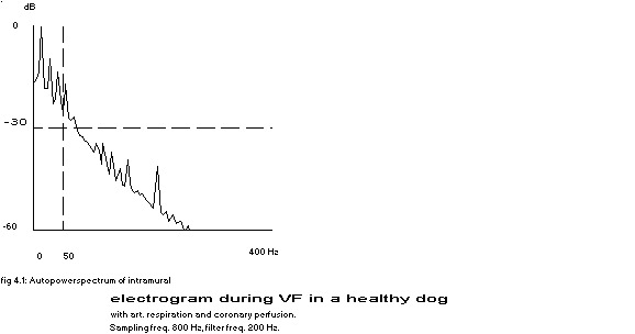
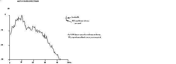
fig 4.1: Autopowerspectrum of intramural electrogram during VF in a healthy dog with artificial respiration and coronary perfusion. Sampling freq. 800 Hz, filter freq. 200 Hz.
Preliminary checks on the frequency content of these signals made clear that almost all power was contained in the frequencies below 40 Hz (see fig. 3.4 and fig. 4.1), so an analog to digital conversion frequency of 100 Hz has been used in this study. The digital values were stored directly on magnetic tape, as explained in the previous chapter.
In general the following procedure was used: a signal of a duration of 40 seconds was analyzed:
- in the time domain by calculation of the amplitude histogram in order to check the stationarity and the type of the probability distribution of the amplitudes of the signal;
- in the frequency domain by Fourier transformation of 20 consecutive blocks of 2 sec’s each and estimating from the ensemble averages the autopower spectra, the autocorrelation function and the autobicoherency spectra.
Although in general all possible care was taken to keep the heart in a good condition, in some cases deliberate changes were made by suddenly changing the mean systemic pressure or by resetting the automatic pump control from constant flow mode to constant systemic pressure mode or to the mode of constant oxygenator weight. These changes in the pumping mode did not really effect the classification of the signals.
No difference has been found between types of electrodes or leads with respect to the classification. The unipolar leads however seem more suitable for an understanding of the results of signal analysis during ventricular fibrillation than the bipolar ones, see the previous chapter. For a meaningful analysis of signals these should be stationary and although Oppenheim and Schafer (1975) state: “In practice, it is common to assume that a given sequence is a sample sequence of an ergodic random process”, attempts have been made to check the assumptions of stationarity and ergodicity; the results are reported in the paragraphs upon histograms, autocorrelation function and auto power spectra. In total 888 signals were analyzed. A summary of this chapter has been published already (Herbschleb 1979).
2 Amplitude histograms
2.1 results
In figures 4.3 – 4.7 examples are given of histograms of the measured voltages. The horizontal axis represents the measured potential in arbitrary units, the vertical one expresses the fraction of samples in a certain voltage class. The continuous bellshaped line represents the best-fitting normal distribution, i.e. the Gauss curve with the same mean and variance as the samples. In an effort to bring some order in the multitude of histogram shapes, all histograms were classified according to the following scheme:
| type | figure | percentage |
|---|---|---|
| unimodal symmetric | 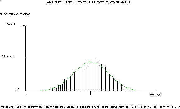 fig.4.3: normal amplitude distribution during VF (ch. 5 of fig. 4.19) 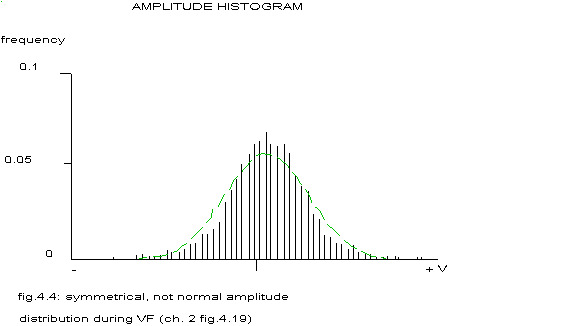 fig.4.4: symmetrical, not normal amplitude distribution during VF (ch. 2 of fig. 4.19) | 40% |
| unimodal skewed | 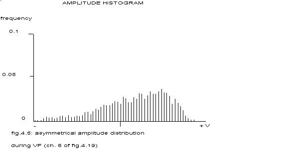 fig.4.5: asymmetrical amplitude distribution during VF (ch. 6 of fig. 4.19) power spectrum in fig. 4.12 | 40% |
| multimodal or uniform | 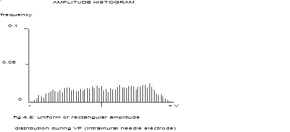 fig.4.6: uniform or rectangular amplitude distribution during VF (intramural needle electrode) | 11% |
| two-peaked | 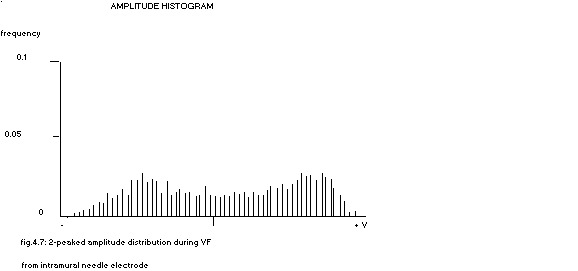 fig.4.7: 2-peaked amplitude distribution during VF from intramural needle electrode | two-peaked |
With the Kolmogorov-Smirnov test (5% level) the class of symmetric histograms could be divided in 15% Gaussian and 85% not Gaussian. As explained already in the previous chapter and the introduction paragraph of this chapter, all histograms were formed from 4000 samples (100 samples per second times 40 seconds). If the analyzed signal is stationary, then these histograms can be considered as a good approximation to the distribution function of the amplitude. In most experiments signal analysis has been repeated at varying intervals, without changes in the electrode arrangements, making it possible to see whether the distribution function is independent of time, a prerequisite for a stationary signal. The next table summarizes how often a certain type of histogram has been followed later in time by the same or another type from the same electrode.
| \ | to | total | ||||
|---|---|---|---|---|---|---|
| unimodal symmetric | unimodal skewed | multimodal or uniform | two-peaked | |||
| from | unimodal symmetric | 183 | 55 | 9 | 5 | 252 |
| unimodal skewed | 62 | 191 | 20 | 19 | 292 | |
| multimodal or uniform | 7 | 21 | 47 | 4 | 79 | |
| two-peaked | 6 | 24 | 5 | 33 | 68 | |
| total | 258 | 291 | 81 | 61 | 691 | |
In many cases the signals could be considered as stationary in this aspect. Moreover, the fact that the row totals are almost equal to the column totals, shows that no systematic trend from one type of histogram to another was present. In two experiments the mean systemic blood pressure has been varied by changing the parameters of the automatic pump control. The results are summarized in table 4.2. There is no clear pattern of dependency of histogram types upon the systemic pressure.
| exp | mm-Hg | unimodal symmetric | unimodal skewed | multimodal or uniform | two-peaked | total |
|---|---|---|---|---|---|---|
| A | 32 | 15 | 15 | 0 | 0 | 30 |
| A | 40 | 17 | 5 | 0 | 8 | 30 |
| A | 50 | 29 | 1 | 0 | 0 | 30 |
| B | 50 | 1 | 7 | 4 | 1 | 13 |
| B | 60 | 0 | 7 | 20 | 12 | 39 |
| A | 67 | 22 | 8 | 0 | 0 | 30 |
| B | 70 | 6 | 34 | 22 | 16 | 78 |
| A | 80 | 2 | 0 | 0 | 0 | 2 |
| B | 80 | 7 | 22 | 9 | 1 | 39 |
| B | 90 | 7 | 26 | 5 | 1 | 39 |
| B | 100 | 3 | 16 | 12 | 8 | 39 |
| total | 109 | 141 | 72 | 47 | 369 | |
2.2 discussion
No reference has been found in literature to the amplitude distribution of the electrogram during ventricular fibrillation. The classification used in this paragraph is rather subjective and ad hoc, lacking an a priori theoretical base to expect certain types of histograms, with the exception of the Normal amplitude distribution. The last type has been found in only 15% of the cases, so in general the electrograms during ventricular fibrillation cannot be considered as normally distributed white noise. Histograms have been found of intermediate type, so classification became somewhat arbitrary.
All 888 histograms have been classified without reference to other information like spectra, histograms of neighbouring electrodes or previous histograms of the same electrode. The numbers in table 4.1 may be considered an indication of consistent histogram classification.
Maybe the whole classification is lacking any significance, as will be explained in chapter VI.
The procedure of recording the signals upon analog tape and replaying them on different recorders for analog-digital conversion has introduced some DC offset, so the mean of the histograms will differ somewhat from zero.
3 Autocorrelation function
3.1 results
The autocorrelation function has primarily been estimated in order to check the assumption of independence between successive blocks in the signal. The confidence interval as plotted in the spectra is based upon the Bartlett averaging method of independent blocks, i.e. no correlation should exist over intervals longer than 2 sec’s for the cases mentioned in this study. Although the pilot studies indicated that the autocorrelation function was damped within 1.5 seconds, so a blocklength of 2 seconds looked reasonable, later experiments showed that sometimes the autocorrelation function would not damp at all (higher than 0.9 after 2 sec’s). Enlarging the blocks would imply lesser blocks for averaging and thus a larger variance of the spectral estimates or a longer total duration of the signal, hoping that the signal would remain stationary over periods much longer than the 40 seconds chosen for this study. Especially the cases where the autocorrelation function was higher than 0.75 after 2 sec’s did not give much hope that the goal of independence between blocks could be reached. For this reasons the originally chosen method of averaging over 20 blocks each of 2 seconds duration was adhered to, but the confidence intervals plotted in the spectra (especially those with sharp peaks) should be taken with a pinch of salt.
The next table indicates the distribution of the estimated autocorrelations after 2 seconds over 4 classes:
classification of autocorrelation functions
| r after 2 s | number | perc. | examples | references |
|---|---|---|---|---|
| r = 0 | 472 | 53 | ||
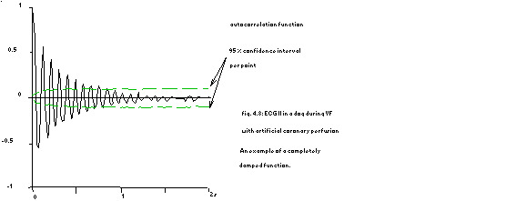 fig. 4.8: ECG II in a dog during VF with artificial coronary perfusion An example of a completely damped function. | ||||
| 0< r <=0.75 | 325 | 37 | amplitude histogram in fig. 4.5 power spectrum n fig. 4.12 | |
 fig.4.9: bipolar epicardial electrogram channel 6 of fig. 4.19 incompletely damped: r=0.71 after 2 s | ||||
| 0.75< r <=0.9 | 45 | 5 | amplitude histogram in fig. 4.6 | |
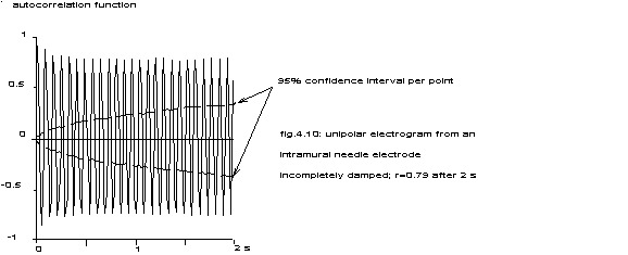 fig.4.10: unipolar electrogram from an intramural needle electrode incompletely damped; r=0.79 after 2 s | ||||
| r >0.9 | 46 | 5 | ||
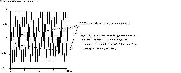 fig.4.11: unipolar electrogram from an intramural electrode during VF undamped function (r=0.94 after 2 s) note typical asymmetry |
3.2 discussion
The division into the two intermediate classes is rather arbitrary, as all damping factors together really form a continuum, but the first class of damped functions and the last class of almost undamped functions are self-evident.
Three remarks should be made about the appearance of the estimated autocorrelation function.
- the clear periodicity in the autocorrelation function corresponds to the first peak in the auto spectrum. Compare fig. 4.9 with fig. 4.12. This periodicity has already been noted by Angelakos and Shepherd in 1957. (Angelakos 1957) In contrast Aubert et al (Aubert 1982) conclude that the ECG during ventricular fibrillation is from a mathematical point of view random, because their autocorrelation function discloses no periodicity. These authors , however, did not analyze purely ventricular fibrillation, but the transition from tachycardia to fibrillation, so their conclusion about the character of ventricular fibrillation is ill-based.
- the autocorrelation function is considered as damped, if the function remains between the indicated 95% confidence lines. The fact that the function still shows a periodic component, is caused by the strong correlations between the autocovariances of a series with moderately strong correlations between the elements of that series (Jenkins and Watts, 1968 p. 185).
- the clear asymmetry in the plotted autocorrelation function – the positive values are higher than the absolute values of the negative r’s – especially in the undamped functions, is explained by the fact that in most cases the autocorrelation function can be thought of as the sum of three cosines:
r(t’)=F(t’)·(A·cos(f·t’)+B·cos(2f·t’)+C·cos(3f·t’))
where A+B+C=1; A,B,C>0
F(0)=1; F(t’) monotone not-increasing
for the autocorrelation function and the autospectrum form a Fourier transform pair and the auto spectrum contains in these cases mostly two higher harmonics of the basic fibrillation frequency (see the following paragraphs). The above equation can be rewritten as:
r(t’)=F(t’)·((A-3C)·cos(f·t’)+2B·cos2(f·t’)+4C·cos3(f·t’)-B)
This function reaches its maximum at cos(f·t’)=1: rmax=F(t’)·(A+B+C); the minimum is reached at cos(f·t’)=-1: rmin=F(t’)·(-A+B-C). In the case that F(t’) does not decrease too quickly a maximum is always higher than the absolute value of the neigbouring minima.
4 Autopower spectra
4.1 results
Figures 4.12, 4.13 and 4.14 give examples of the autopower spectra of electro(cardio)grams during ventricular fibrillation. As explained in the introduction these spectra were estimated by averaging the periodograms of 20 consecutive blocks of 200 samples each, with a sample interval of 10 ms. Thus the resolution is 0.5 Hz and the highest frequency represented is 50 Hz. The anti-aliasing filter was set at 30 Hz. The vertical axis represents the power (proportional to the square of the amplitude) on a logarithmic scale. The horizontal bar of the cross in the upper right corner indicates the bandwidth, the vertical bar the 95% confidence interval per frequency band.
Characteristic for ventricular fibrillation is a high, relatively narrow peak around 12 Hz (range: 9-13 Hz) in the dog and around 6 Hz in man, followed by peaks at frequencies two, three, four etc times higher than the first one. Mostly three clear peaks were seen.
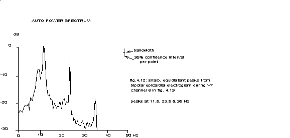
peaks at 11.5, 23.5 & 35 Hz
channel 6 in fig. 4.19
correlation in fig. 4.9
histogram in fig. 4.5
zoomed spectrum in fig. 4.31
In about 25% of all signals analyzed low peaks were seen at the half frequencies in between the high peaks. In chapter VI the possible significance of these peaks will be discussed. Only 35 cases (4%) have been found with just one narrow peak in the auto spectrum.
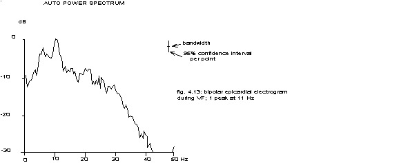
1 peak at 11 Hz
In only 14 cases (2%) autopower spectra have been found without narrow peaks, but with a broad peak like e.g. low-pass filtered white noise.
a spectrum without a clear, narrow peak
4.2 discussion
The auto spectrum of an electro(cardio)gram during ventricular fibrillation differs from such a spectrum during other rhythms in having most of the power concentrated in a few more or less equidistant peaks, see: Nygårds 1977, Hulting 1979, Martín 1981, Forster 1982, Cosín 1982 and Herbschleb 1980a. The spectra published by Nygårds & Hulting (1977) and Hulting (1979) of ventricular fibrillation in patients agree in general with the most common type of spectrum in this study. These authors diagnose ventricular fibrillation if the spectrum contains above 4 Hz a frequency peak with 85% of all power. The spectra published by Martín et al (1981), Forster and Weaver (1982) and Cosín et al (1982) do mostly show just one peak, as they use a linear vertical scale. None of these authors applied ensemble averaging, so the variability in their spectra is much higher than the variability in the spectra used for this study.
Contrary to accepted views (e.g. Scher 1976 or Zipes 1975) on the random nature of the ECG during ventricular fibrillation, the spectra mentioned above indicate a very high regularity. In chapter VI, par. 5 a method to estimate the degree of regularity will be given.
The following authors seem to support the hypothesis of randomness of ventricular fibrillation by their experimental results. Agizim et al. (1976) published a spectrum of the ECG during ventricular fibrillation in a dog looking like the spectrum of white noise; no explanation could be found for this controversy. (Agizim 1976). Tabak et al (1980) analyzed the spectrum of the ECG during ventricular fibrillation in dogs without coronary perfusion. In the first stadium they saw a peak at 12 Hz and as they estimated the spectra up to 25 Hz, no higher harmonics could be found. In later stadia they saw 2 peaks at 4.5 and 9 Hz, but as the hearts of their animals must have been already greatly anoxic, these results cannot be compared with the spectra described in this chapter. (Tabak 1980).
Nolle et al. (1980) estimated the power spectrum of the ECG during ventricular fibrillation in patients of episodes with a duration of maximal 4.096 seconds (1024 samples). When there were not enough data, the samples were augmented with zero’s; a very questionable procedure, see appendix A. Moreover, no averaging or smoothing had been performed, so their results in ventricular fibrillation/tachycardia (sic) do not look very useful. (Nolle 1980). The ill-based conclusion of Aubert et al (1982) about the random character of the ECG during ventricular fibrillation has already been dealt with in the preceding paragraph.
Most of these results seem to indicate a very rapid, repetitive phenomenon during ventricular fibrillation, viz. 12 Hz or 720 “beats” per minute in dogs and 6 Hz or 360 “beats” per minute in men. These frequencies are much higher than can be reached by a beating heart, (in chapter 6, par. 3 an explanation will be attempted) but are in accordance with the emphasis in the older literature put upon the high, rather regular, repetititon rate of “beats” during ventricular fibrillation. In 1850 Hoffa & Ludwig mention 84 “heartbeats” in 8.34 seconds (10.1 Hz) in fibrillating rabbit hearts. Hoffa 1850. McWilliam (1887), Rothberger & Winterberg (1914,1916) and Kisch (1921) also drew attention to this high repetititon rate (McWilliam 1887, Rothberger 1914, Rothberger 1916 and Kisch 1921).
In order to get an idea of the stability of the heart during ventricular fibrillation the mean fibrillation frequency in long lasting experiments has been plotted in the next figure.
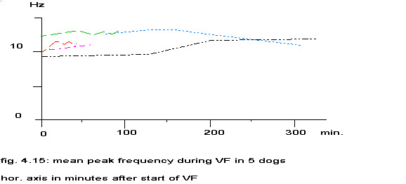
hor. axis in minutes after start of VF
No trends in fibrillation frequency have been found in these experiments, although prominent shifts have been found in several experiments described in chapter XI.
The various mean systemic blood pressures do not affect the fibrillation frequency, see the next figure.
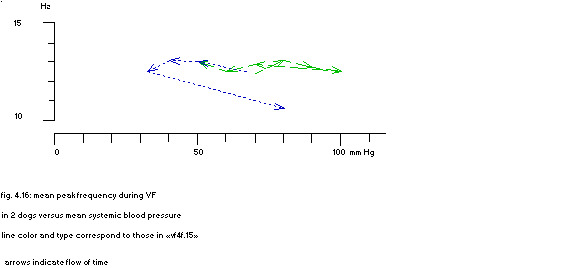
arrows indicate flow of time
line color and type correspond to those in fig. 4.15
5 Auto bicoherency spectrum
The autobicoherency spectrum expresses the coherency between the phases of the frequencies f1, f2 and f1+f2 in a measure between 0 and 1, but only if the analyzed signal fulfils certain conditions like normality. The signals mentioned in this chapter are in majority not normal (par. 2) and then the autobicoherency may rise to infinity. See appendix D and Dumermuth 1971. These difficulties were overcome by setting the amplitude component of all frequency bands equal to 1 in the complex spectrum.
Only those equidistant peaks in the auto power spectrum were considered as true harmonics of each other if their autobicoherency rose above a confidence level of 0.999 for white noise. Of the 888 analyzed electro(cardio)grams 839 showed narrow, equidistant peaks in their power spectrum, see the previous paragraph. Of these 839 signals 251 or 30% did not show any autobicoherency above the significance level. The peaks in the spectrum of the remaining 588 signals were true harmonics of each other. In the separate bicoherency page examples are given of autobicoherency spectra, where only the values above the significance level of 0.5687 have been plotted (see also appendix D).
Figure 4.17 shows that, albeit low, there is a coherency between 11.5, 12 and 23.5 Hz and between 11.5, 23,5 and 35 Hz, which means that the peaks in the power spectrum fig. 4.25 of 11.5, 23.5 and 35 Hz are harmonics of each other. In fig. 4.18 an example is given of high autobicoherencies. The peaks in the power spectrum fig. 4.12 of 23.5, 35 and 47 Hz are clearly higher harmonics of 11.5 Hz.
As could be expected, the majority of the signals without significant autobicoherencies are in the class of symmetric histograms with a damped autocorrelation function. In paragraph 8 a summary of the results of the paragraphs 2, 3, 4 and 5 is given in the form of a table.
6 Diversity of signals from one fibrillating heart
The preceding paragraphs could give the impression of a bewildering variety of types of ventricular fibrillation. This paragraph will show the variety of signals from one fibrillating heart, indicating that the signal analytical types of ventricular fibrillation do not imply different underlying syndromes.
electrode in fig. 3.2
analysis of experiment in tabular form
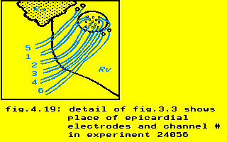
In figure 4.19 is indicated where the epicardial electrode with 13 terminals plus 4 single epicardial electrodes had been attached to the epicardium of the right ventricle. In this experiment bipolar electrograms were recorded as shown in fig. 4.19; for illustrative purposes the channels of the analog recorder have been indicated. ECG lead II was recorded on channel 7. Channels 4, 5, 6 and 7 will be used to illustrate the variety of signals arising from a small area of a fibrillating heart.
The bewildering diversity can be studied through the following table.
| type of analysis | channels | ||||
|---|---|---|---|---|---|
| 2 | 4 | 5 | 6 | ECG | |
| TV-raster plot | fig. 3.5 | fig. 3.6 | fig. 3.7 | ||
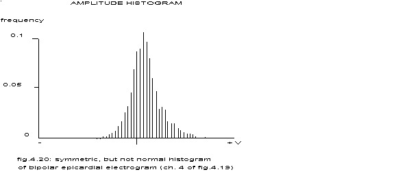
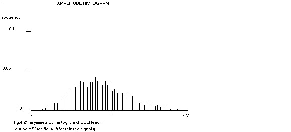
| amplitude histogram | fig. 4.4 | fig. 4.20 | fig. 4.3 | fig. 4.5 | fig. 4.21 |
| auto power spectrum | fig. 4.25 | fig. 4.26 | fig. 4.12 | fig. 4.27 | |
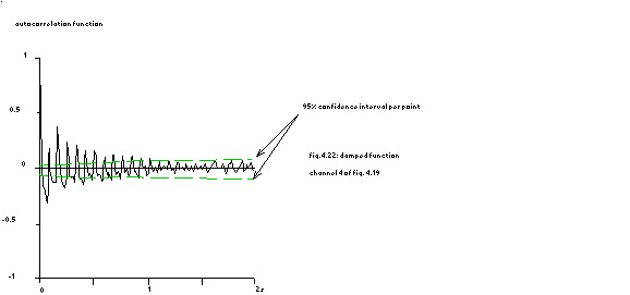
| auto correlation | fig. 4.22 | fig. 4.23 | fig. 4.9 | fig. 4.24 | |
| auto bicoherency | fig. 4.17 | fig. 4.29 | fig. 4.18 | fig. 4.28 | |
| zoom FT | fig. 4.31 | fig. 4.31 | fig. 4.31 | ||
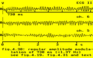
| signal plot | fig. 4.30 | fig. 4.30 | fig. 4.30 | ||
The histograms of channels 4, 5, 6 and 7 (ECG) show respectively a symmetric (but not Normal), a Normal, and two asymmetrical amplitude distributions simultaneously. The autocorrelation function of channels 4 and 5 is damped after 1000 resp. 1750 ms. the autocorrelation of channel 6 reaches a value of 0.71 after 2 sec’s and that of channel 7 is almost damped (0.21) after 2 sec’s. Even the basic fibrillation frequency is not the same in this small area. The spectrum of channel 4 consists of peaks at the frequencies 11.5, 23.5, 35 Hz (like channel 6) and – less clearly – at the frequencies 6, 17.5 and 29 Hz. The spectrum of channel 5 however shows a clear peak at a frequency of 10.5 Hz and much less pronounced a peak at 20.5 Hz. In the ECG (channel 7) both frequencies seem present, although the size of the 95% confidence interval as plotted in the right upper corner precludes such a conclusion. The next paragraph will show that this ECG can be considered as the electrical summation of signals with a basic frequency of 10.5 and 11.5 Hz. The bicoherencies indicate that the frequencies of 23.5 and 20.5 Hz are really higher harmonics of the basic frequencies. The conclusion is that different “types” of fibrillation are simultaneously present in one fibrillating heart and that these types are independent of the electrodes used.
power spectrum in fig 4.25
power spectrum in fig. 4.27
amplitude histogram in fig4.20
power spectrum in fig. 4.25
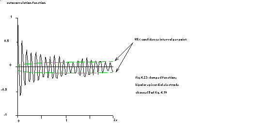
bipolar epicardial electrode, channel 5 of fig. 4.19
amplitude histogram in fig4.3
power spectrum in fig. 4.26
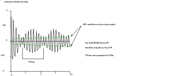
730 ms corresponds to 1.37 Hz, see fig4.31
amplitude histogram in fig. 4.21
power spectrum in fig. 4.27
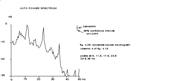
peaks at 6, 11.5, 17.5, 23.5, 29 & 35 Hz
correlation in fig. 4.22
histogram in fig. 4.20
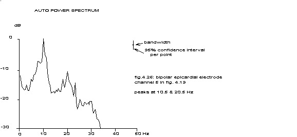
peaks at 10.5 & 20.5 Hz
correlation in fig. 4.23
histogram in fig. 4.3
zoomed in fig. 4.31
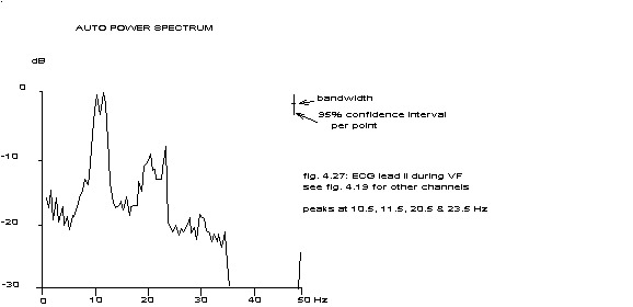
peaks at 10.5, 11.5, 20.5 & 23.5 Hz
correlation in fig. 4.24
histogram in fig. 4.21
zoomed spectrum in fig. 4.31
7 Amplitude pulsation
Characteristic of electrograms during ventricular fibrillation is the regular waxing and weaning of the amplitude. This regularity suggests amplitude modulation or “beating”, caused by the summation of two signals with slightly different frequencies. To avoid misunderstanding within the field of cardiology the technical term “beating” will not be used furthermore in this study.
see channel numbers in fig. 4.19
zoomed spectrum in fig. 4.31
In fig. 4.30 a part is plotted of the signals from the channels 5, 6 and 7 discussed in the preceding paragraph. The pulsation interval of 0.73 seconds has been indicated in this figure. The autospectrum of the ECG fig. 4.27 did not justify the conclusion of two separate peaks, so a higher resolution of the frequency band of 6 – 14 Hz was necessary. This higher resolution has been reached by a technic known as “ZoomFFT” (see appendix F) and the result is shown in fig. 4.31 for all 3 channels mentioned.
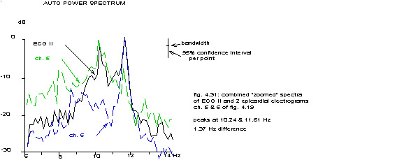
2 epicardial electrograms (ch. 5 & 6 of fig. 4.19
peaks at 10.24 & 11.61 Hz; 1.37 Hz difference
Very clearly the ECG can be considered as the sum of two signals with frequencies of 10.24 and 11.61 Hz; the difference of 1.37 Hz leads to a pulsation interval of 0.73 sec’s. The much more irregular amplitude variations of channels 5 and 6 could be caused by a mixture of amplitude- and frequency modulation, see chapter VIII and appendix E. This pulsation caused by summation of signals with slightly different frequencies has also been demonstrated in other experiments.
8 General discussion and conclusion
All the numbers of signals in different classes of signal analysis as mentioned in the preceding paragraphs have been summarized in table 4.3.
| narrow, equidistant peaks in power spectrum | total | |||||||||
|---|---|---|---|---|---|---|---|---|---|---|
| auto correlation after 2 s | histogram type | |||||||||
| unimodal symmetric | unimodal skewed | multimodal or uniform | two-peaked | |||||||
| bicoherency | bicoherency | bicoherency | bicoherency | |||||||
| not sign. | significant | not sign. | significant | not sign. | significant | not sign. | significant | |||
| r = 0 | 118 | 73 | 59 | 132 | 1 | 23 | 1 | 20 | 427 | |
| 0 < r <= 0.75 | 50 | 83 | 11 | 106 | 7 | 36 | 1 | 27 | 321 | |
| 0.75 < r <= 0.9 | 4 | 22 | 1 | 8 | 1 | 9 | 45 | |||
| r > 0.9 | 5 | 22 | 1 | 18 | 46 | |||||
| one narrow peak in power spectrum | ||||||||||
| auto correlation after 2 s | histogram type | |||||||||
| unimodal symmetric | unimodal skewed | multimodal or uniform | two-peaked | |||||||
| r = 0 | 21 | 10 | 31 | |||||||
| 0 < r <= 0.75 | 3 | 1 | 4 | |||||||
| no narrow peaks in power spectrum | ||||||||||
| auto correlation after 2 s | histogram type | |||||||||
| unimodal symmetric | unimodal skewed | multimodal or uniform | two-peaked | |||||||
| r = 0 | 7 | 7 | 14 | |||||||
| total | 359 | 353 | 98 | 78 | 888 | |||||
a 2-dimensional representation of a 4-dimensional classification scheme
These numbers would have been quite different if the four ways of classification (histogram, autocorrelation function, autospectrum and autobicoherency) were independent of each other. Clearly this is not the case, compare e.g. the overall percentage of 70 for the significant bicoherencies par. 5 with the actual distribution in table 4.3. In general the table shows – not surprisingly – a tendency for more sinusoidal signals (according to histogram type) towards a strong autocorrelation, autobicoherency and narrow, equidistant peaks in the spectrum, but unexpected combinations do occur. The autospectrum of most signals contains two or more equidistant narrow peaks, mostly bicoherent, which points into the direction of a rather regularly repeated electrical phenomenon (see chapter VI, par. 4 and appendix E). The coefficient of variation (standard deviation / mean) of the intervals between these regular phenomena will in this case be smaller than 0.09. However, the repetition frequency of 12 Hz (720 bpm) in dogs and 6 Hz (360 bpm) in man is much higher than can be reached by a normally beating heart. Sano et al Sano 1958 did report such high repetition rates in single myocardial fibers, but the absence of a calibration line in their figures plus the clear alternans in the shape of their complexes sheds some doubt on the validity of their measurements. On the other hand Trautwein and Zink Trautwein 1952 published action potentials during ventricular fibrillation in frogs, cats and dogs that looked rather normal. The repetition rate during ventricular fibrillation was slightly higher than the rate of a ventricular tachycardia and the highest rate they published was 260 bpm in dogs. Unfortunately these authors did not give data on the external ECG, contrary to Sano c.s. who showed a synchrony between the ECG and the action potentials. Nevertheless the results of Trautwein and Zink fit the known physiological properties of the heart of the dog much better. The highest rate of the heart of Beagles in treadmill tests has been reported as 303 ± 17 bpm (= 5.05 Hz) Young 1961. Moulopoulos et al (Moulopoulos 1965) reported a highest stimulated ventricular rate in dogs of 280 bpm (= 4.67 Hz). The effective refractory period of the ventricular myocardium in dogs has according to Han et al (Han 1966) a range of 177-195 ms at a repetition interval of 200 ms (300 bpm) and according to Amlie (Amlie 1978) a range of 137-151 ms. These values correspond with the length of the action potentials as reported by Trautwein and Zink in 1952 (110-140 ms) and by Russell et al in 1979 (182 ± 9 ms), (Russell 1979) but preclude repetition rates above circa 450 pm (9 Hz) in dogs, unless we assume a drastic change in the physiological properties of the myocardial cells instantaneously at the transition from normal beating to electrically induced ventricular fibrillation.
This controversy can be solved by another assumption. In paragraph 4 of this chapter the fact has already been mentioned that in 25% of all spectra subharmonic peaks were seen, which can arise if the measured phenomena alternate in shape and/or size. Maybe the repetition rate of individual cells is lower than the overall rate measured by extracellular electrodes. In order to get some insight in this possibility, model studies have been performed. See the next chapter for the models and chapter 6 for a re-evaluation of this chapter in the light of the results of chapter 5.
Hier ontbreekt nog het e.e.a.
Pagina IV-26 t/m IV-30 van boek staan niet op de website. Kan Han tekst aanleveren?