1 An anecdote
Years ago I belonged to a group of young biologists working in a Dutch independent research institute, situated at the most magnificent street of Europe (according to the most remarkable man I ever met). At coffee break we used to discuss politics, philosophy, child raising, science, in short: we were improving the world. One of us was strongly opposed to scientific theories. He argued: a true scientist performs an experiment and writes down his observations. To pull his leg I asked him if he also noted the taillength of his mice. Of course not! he exclaimed indignantly, the taillength has nothing to do with my experiments with oestrogens. I pointed out that his conviction was just a theory, and worse: a wrong theory. In general the taillength of mice depends upon the temperature difference between their body and the environment in which they grow up. Oestrogens influence the mean body temperature, the environmental temperature was kept constant, so administering oestrogens to immature mice will influence their taillength. My opponent was furious and walked out (for already a long time he is a well-known university professor).
A few months later I met in the corridors one of the other biologists carrying bunches of mouse tails. Yes, he said, you were quit right. This is the quickest test to see whether the oestrogen administration had effect, before we do the complicated and lengthy research with the electron microscope.
2 A philosophical introduction
2.1 The role of models and theories
This is not intended as an introduction into the philosophy of science. For good introductions see Popper 1965 , Nagel 1971 and Harr, 1981 .
The anecdote (it truly happened) illustrates what I want to say about models and theories in the natural sciences. With “model” is not meant a formal, sentential model as used in logic and mathematics, but an iconic model, i.e. a real or imagined thing and process which is similar to other things and processes in various ways, and whose function is to further our understanding. A model is always a restriction, compared to the real world, but its limitations are known. Violating the postulates of a model invalidates any interpretation of the outcome from the model. If a researcher is not aware of the models and theories his work and ideas are based upon, than ridiculous scenes as sketched above may occur or worse.
A reason to use models is to simplify, so calculations and predictions become possible. Using all information about a myocardial cell for all cells in the heart, would make any calculation intractable Scher 1979 (page 372).
2.2 Weeding out erroneous experimental results
In research almost always some selection of material and results is necessary because of errors made in difficult experiments. There lurks however a big danger in the selection process: what is an error? In terms of models: different models may predict contradictory results; an error according to one model might be the looked after result according to an other model.
The researcher convinced of orderly travelling wavefronts during ventricular fibrillation selects frames 1 – 13 from fig. 7.7 to prove his point of view. A constantly changing wavefront (both in speed and in direction) is proven with frames 13, 14, 15 and 16 of fig. 7.7 and a careful selection of frame 20 of fig. 7.7 shows the long looked after circular front in a small space.
In no way is the use of Ideker’s work – Ideker 1981 – in chapter IX, par. 3 meant as criticism. His experimental setup is much better than mine, so I took the freedom to use his figures to show that an other point of view would give an other interpretation of the same observations.
3 A four-level model of fibrillation
3.1 Introduction
In all discussions about theories and models of ventricular fibrillation I never was able to clearly explain the concept of a multilevel model. To understand my study, however, this is of crucial importance. The latest model of ventricular fibrillation that came to my knowledge, uses an array of 2500 discrete elements Mitchell 1992 . This model shows several aspects of ventricular fibrillation, but there is no theoretical connection between one such an element and the microscopical structure of the myocard. The model is more or less comparable to my level 3.
The best explanation of levels is found in the …Ant Fugue, one of the dialogues between Achilles, Crab, Anteater and Tortoise Hofstadter 1980 . The anthill is not considered as a collection of randomly wandering ants, but as an information processing entity; the dumb ants are just elements of the system. Severely disturbing the colony does not change or kill the individual ants, but could completely destroy the old anthill system. A new “hill” will be born in short time without any resemblance to the old system. The fibrillating heart is not – in my opinion – the same old heart with suddenly altered myocardial cells, but a new heart with the same old cells in a new functional configuration. The anatomy, of course, does not change.
The highest level model of the heart is an old one already of van der Pol 1929 ; this model never shows anything like ventricular fibrillation, but modelling the atrio-ventricular node as a relaxation oscillator (like level 1 in chapter VIII, par. 2 ) clarified much of the arrythmias originating from this node van der Tweel 1986 .
3.2 Level 0
The lowest level in my model is the myocardial cell, described as a simple system with a finite number of internal states which may be changed by external inputs; without interference from the outside the states succeed each other in course of time until a quiescent state has been reached. The cells do not necessarily possess pacemaker capabilities. See chapter V, par. 3 for details.
3.3 Level 1 – its history
Our first models were based upon models found in the field of epidemics Waltman 1974 using the following analogy:
- msec – day
- quiescence – susceptibility
- excitability – exposure
- activity – infectivity
- refractoriness – recovery
The classical approach started with Kermack and McKendrick in 1927 Diekman 1978 and does not consider loss of immunity i.e. return from the class “recovered” to the class “susceptible”. Nevertheless the statement from 1927: “ An epidemic, in general, comes to an end, before the susceptible population has been exhausted“, is important because it points to the probability that in one cycle of ventricular fibrillation some cells will remain quiescent. No sustained activity is found in these models of course. Good reviews are available Bailey 1975 and Diekman 1978 .
Waltman published in 1974 his analysis of models of epidemics with recurrent infections. His assumptions, particularly that of a constant population, fit ventricular fibrillation better than epidemics. Just like in the first mentioned neuronal networks all elements are supposed to have a chance of making contact, which is even in a very small area in the myocardium not likely. Very important in his model is the threshold. An individual becomes only then infectious after exposure if during a certain time interval enough contacts with infectives have been made. Contrary to the statements in the classical theory, he was not able to prove mathematically the existence of a periodical solution, but simulations of his model exhibited a periodical change in the number of infectives after the introduction of the appropriate number of infectives into the population. The length of the period was equal to the sum of the lengths of the states: exposed, infective and recovered. Intuitively there is a resemblance to modeling by the logistic equation, especially if time delays are introduced.
dN/dt = rN[1-N(t-T)/K]
where: N = population size
t = time
r = factor representing response to disturbance
T = time lag
K = magnitude of equilibrium population
Long delays with regard to the response time of the system lead to a so-called Hopf bifurcation and consequently to oscillations through stable limit cycles. For an introduction see May 1976a and for an extensive treatment see Iooss 1980 . Later the existence of a periodic solution for these epidemic models was proven Gripenberg 1980 .
3.4 Level 1 – Chaos?
Considerable interest has arisen in the type of equations in chapter VIII, par. 2.3 since the publication of May May 1976b and for a review see Hofstadter 1981 . The form of equation 8.11 is plotted in the next figure for several thresholds.
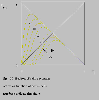
Clearly the steepest part of the function approaches a slope of -1, so the system will always tend to an equilibrium with p(t+1)=p(t). The slope will never exceed -1, so this equation will never lead to chaos, see Cvitanovic 1984 , Feigenbaum 1980 , Devaney 1986 and Gumowski 1980 , in accordance with the signal analysis presented in this study and contrary to the accepted claim of chaos during ventricular fibrillation, see WHO 1978 and Gleick 1987 (page 284).
The “thresholds” of figure 12.1 are not the thresholds for the individual cells, but these thresholds minus the environmental noise ( equation 8.12 ). Changes in the activity of the environment of the system will push the system from one curve to another, so even if equilibrium has been reached, the probability of becoming active fluctuates with the environmental activity. Furthermore the curves of fig. 12.1 represent probabilities of becoming active, so any realisation of this system will also show stochastic variations.
The Box-Jenkins approach failed (as mentioned in chapter III, par. 4.4 ) because equation 8.12 contains powers of p(t), so the system is not linear.
At thresholds 10, 15 and 20 the curves show an instable point, which means that if a certain level of activity has been passed, the system becomes silent. With a threshold of 25 or 30 no persistent activity is possible. At a threshold of 1 or 5 the system can oscillate between high and low activity, but gradually the equilibrium will be reached. The higher the threshold, the faster the equilibrium is reached. This can be considered as an explanation for the behaviour of the model of chapter V ( topolt ), for some of the experiments of chapter XI and for the link between ventricular tachycardia, flutter and fibrillation. At a threshold of 15 not all cells will become active within one repetition period, as the probability of becoming active in equilibrium is lower than 0.5. In this case the irregularity of a realisation of this system will be higher than at lower thresholds. Any manipulation will disturb the equilibrium and if at the same time the threshold is suddenly lowered (by anoxia and/or higher environmental noise), a tachycardia-like activity can originate, that will revert to fibrillation if the original situation is more or less restored. See chapter XI, par. 2 .
The chaotic or irregular dynamics as described for cardiac cells Guevara 1981 and for electronical and mathematical non-linear oscillators Guevara 1982 and Testa 1982 (plus the books mentioned above) always show period doubling, tripling, etc., but never halving of the original period. These dynamics bear no relevancy to my analysis of ventricular fibrillation.
3.5 Level 1 – the Fractal
The definitive model in chapter V, par. 3 is described as a cellular automaton, i.e. a uniform array of many identical cells, or sites, in which each cell has only a finite number os possible states and interacts only with its immediate neighbours. For a non-mathematical introduction Hayes 1984 . The word ‘cell’ does normally not mean cell in an anatomical sense; in my model ‘cell’ means both myocardial cell and element of a cellular automaton. Developmental systems can be described as cellular automata in an infinite cellular space where each cell has the capacity to generate offspring – depending on its state and the state of its neighbours Lindenmayer 1975 .
The system proposed by Lindenmayer in 1968 as a foundation for an axiomatic theory of development is nowadays known as L-system. The model of chapter V could be described as a 3-dimensional L-system, but that did not seem to give more insight Mayoh 1974 .
The growth of a filament of algae with branches in a 2-dimensional cellular space can be compared to the development of an ECG in time, if one considers one dimension of that cellular space as the time dimension. The L-system used to describe the development of a ‘normal’ ECG will be found in file: norm_ecg.ltl and that of the transition of ‘tachycardia’ into ‘fibrillation’ in file: vf_ecg.ltl . For an explanation of the formalism used see appendix G . Leaving out the graphics symbols the explanation of these L-systems is:
cz -> nnnnnzaz -> ooooozaz -> ooooozbz -> ooooozcz -> oooooznnnnnzaz etc.
i.e. after 3 computational steps (5 timesteps) the system repeats itself
Shortening the number of timesteps after ‘c’ will create a tachycardia deteriorating into fibrillation; state ‘c’ could be compared to the atrio-ventricular node impulse, once the fibrillation starts, the system never enters state ‘c’ again.
cz -> nnnnzaz -> oooozaz -> oooozhz -> oooozkz -> oooozynnnnzaz ->
oooozyoooozaz -> oooozyooooziz -> oooozyoooozlz -> oooozyoooozxnnnnzaz
-> oooozyoooozxoooozaz -> oooozyoooozxoooozjz -> oooozyoooozxoooozmz
-> oooozyoooozxooooznzaz -> oooozyoooozxoooozozaz ->
oooozyoooozxoooozozdz -> oooozyoooozxoooozozgz -> oooozyoooozxoooozozpz
-> oooozyoooozxoooozozqz -> oooozyoooozxoooozozez ->
-> oooozyoooozxoooozozez etc
In words: too fast a rhythm will not activate all myocardial cells; half a cycle later the rest gets activated, activates in its turn part of the cells again half a cycle later, etc.
The graphical interpretation of this L-system is a fractal Prusinkiewicz 1989 . .
3.6 Level 2
At this level we consider the level-1 clusters as non-linear weakly coupled relaxation oscillators. There exists a large number of publications in this field, so I only refer to those publications that somehow influenced my thinking: Kuramoto 1975 , Ashkenazi 1978 , Gollub 1978 , Pavlidis 1978 , Winfree 1979 , Grasman 1984a , Grasman 1984b and Keith 1984 .
At this level chaos is possible in the sense of non-periodic dynamics, but our signal analysis did not show really chaotic signals.
The program vfsum level 2 simulates this level.
3.7 Level 3
This level comprises the whole ventricle. Representing the state of the ventricle during fibrillation with the weakly connected relaxation oscillators of level 2 would require an enormous amount of such oscillators. One oscillator represents 1000 myocardial cells, standing for a piece of myocardial tissue of 0.1 by 0.1 by 1 mm. The whole left ventricle of the dog will contain the order of magnitude of 10 million of such oscillators. Simulation of such a number is not feasible, so the program vfsum simulates just a few hundred of oscillators. The distance between these oscillators is in general more than 10 mm, so they can be considered independent, see chapter IX, par. 4 and chapter VII, par. 3 .
4 The future
Based upon our observations and our models some ideas arose for future investigation.
4.1 Start of fibrillation – one untimely pulse
In the experiments described in this thesis ventricular fibrillation has always been initiated by stimulation with an electrical current of 50 Hz. The concept of very rapid pulses driving all myocardial cells in a different phase originated from these experiments. Other ways of exciting ventricular fibrillation have been left out of the model studies in order to avoid even more complicated models. The measurements described in chapter X indicate a large similarity between types of ventricular fibrillation with a different origin. From fig. 12.1 it is clear now that the only prerequisit for ventricular fibrillation is that a group of cells is in antiphase with another strongly connected group. This situation will be reached by one untimely pulse (assuming some variation in electrophysiological properties of neighbouring cells) or by currents leaking from an infarction zone.
The topological model shows this reaction, see chapter V, par. 2.7 .
4.2 End of fibrillation
From the formulas in this chapter three ways of ending ventricular fibrillation can be derived.
- bring all cells in the same phase, as a prerequisite for fibrillation is the presence of two groups of interlaced cells in antiphase. The common practice of defibrillation with a strong direct current is an example of this method. In terms of oscillators this has been named a type 0 phase resetting Winfree 1980 .
- prolong the refractory period of the myocardial cells in respect to their depolarized period. The publication of Smailys et al. Smailys 1981 indicates how 4 out of 15 dogs have been defibrillated by treating them with ultrasound with a frequency of 500 kHz and an intensity of 10 W/cm2, probably by prolonging the refractory period.
The fact that a drug which prevents the start of ventricular fibrillation, does not stop fibrillation chapter XI, par. 4 could be explained as follows. If the drug prolongs the refractory period – the fibrillation frequency decreases from 10.5 to 8 Hz – the probability of getting cells in antiphase diminishes chapter VIII, table 1 . Once however fibrillation is present, the same mechanism will push all cells into one of the possible classes, so the peaks in the spectrum will become much sharper, but ventricular fibrillation does not stop. This assumption should be tested much more extensively. - raising the threshold will make continuation of ventricular fibrillation less probable and at a higher level even impossible, see figure 12.1 . A higher threshold in the model simple means that cells are less excitable and the anti-arrhythmic action of e.g. verapamil could in this way be fitted in the model.
4.3 Weakly connected relaxation oscillators
The aggregates of 1000 cells have somewhat loosely been designated as relaxation oscillators in chapter V. In chapter VIII ventricular fibrillation at large has been described as the effect of coupling a lot of such relaxation oscillators in a threedimensional structure. The formulas of that chapter will make a much more detailed study possible. The period of the oscillator is given by equation 8.10 , and if we read for Nb in equation 8.7 Nb + NE , the influence of the connected oscillators has been defined. NE should of course be seen as a vector, and its magnitude is determined by the size of the contact area between oscillators and the amount of activity within the neighbours (equation 8.12 ) taking into account the length of the active period.
4.4 Conduction or synchrony
The “conduction” of electrical activity from one cell to another in the model of chapter V has been described beautifully by Janse 1980 : “… the small area was activated from different sides, the wavefronts taking tortuous routes, in which incomplete circus movements were much more frequent than complete ones.” The size of electrodes plus the space constant of 1 mm for micro electrodes does not make it possible to follow the fate of an individual cell during ventricular fibrillation, whereas the history of the cells of the model could be followed individually. The concept of a wavefront is not sensible for the model, because the fibrillation is in this case sustained by two groups of cells in antiphase and in that case one cannot tell which group precedes which. The formulas of this chapter indicate how the repetition period is constantly slightly changed under influence of the activity of the environment of a cell, so a cell that seems to precede another one will after a small change of period seem to follow. If one tries to interpret the effects of these changes in period as different directions of a wavefront, very tortuous paths will indeed be found.
Maybe never experiments will be possible to test this part of the model in a real heart and the best one could do is to adhere to the definition of Han for the reentrant activity during ventricular fibrillation: “ focal reexcitation due to the flow of current between adjacent myocardial fibers that are repolarized at grossly disparate times” Han 1971 , in contrast to the circus reentry.
4.5 Regularity
In chapter VI, par. 5 a tentative measure for regularity of ventricular fibrillation was given. The nomograms of appendix E could be used to estimate the regularity, but much more investigations should be made to find out the reliability and clinical significance of this measure.
4.6 Variability in refractory period
In chapter VIII, par. 2.2 the variability in refractory period amongst cells was mentioned. The total duration and frequency of pulses necessary to start ventricular fibrillation maybe indicates this variability, but again: more investigations are required.