1 Introduction
In cahpter IV, par. 6 an example has been given of independently active areas in the heart during ventricular fibrillation. In this chapter an attempt will be made to estimate the size of such independent areas, their stability and to check whether propagated wavefronts are present within coherent areas. The size estimation has been based upon the squared coherency spectrum appendix A. Propagation speeds have been calculated from the phase shifts between coherent signals from adjacent electrodes appendix C. These cross spectra were estimated between the electrodes mentioned in the chapters 3 and 4 during ventricular fibrillation in 11 healthy dogs with artificial coronary perfusion. See also the introduction to chapter IV.
2 Methods used: a justification
2.1 Number of analyzed electrode pairs
Not all possible electrode pairs have been used and table 7.1 shows the distribution of the number of spectra over these dogs.
| dog # | pairs | comment |
|---|---|---|
| 02095 | 95 | These 2552 electrode pairs cannot be considered independent in a statistical sense. This fact should be kept in mind when viewing the histograms in this chapter. |
| 23095 | 99 | |
| 06016 | 180 | |
| 27016 | 297 | |
| 28016 | 627 | |
| 18036 | 243 | |
| 12056 | 336 | |
| 24056 | 136 | |
| 18116 | 213 | |
| 03037 | 288 | |
| 04117 | 48 | |
| 2552 | total |
2.2 Squared coherency spectrum
The squared coherency spectrum, which will be denoted simply as coherency (K2) in the rest of this chapter, plays the role of a correlation coefficient between two signals, defined at each frequency band. If there exists no correlation at all at a certain frequency, the coherency is zero. The coherency equals 1 if the two signals behave identically at the frequency band considered. As the coherency is a stochastic variable, a test has to be applied in order to see whether the estimated coherency differs from zero or not. Because of the large amount of possible electrode pairs in one experiment, a significance level of 0.001 has been chosen. Two electrodes will be called coherent, if the coherency between their signals at the basic fibrillation frequency is so high that the critical value associated with this level is surpassed. The basic fibrillation frequency is the frequency with the highest peak in the autopowerspectrum, although in the preceding chapters reasons were given to assume that the individual myocardial cells run at half that frequency. The formulas to estimate the coherency and its critical value are given in appendix A.
The coherencies discussed in this chapter are based upon a division of the signals in 20 consecutive blocks, so the critical value is 0.2113. For illustrative purposes the coherencies have been classified into three classes:
| 1 | 0.2113 < K2 <= 0.5322 |
| 2 | 0.5322 < K2 <= 0.8161 |
| 3 | 0.8161 < K2 <= 1. |
An area will be called a coherent area if all electrodes within that area are coherent. By adding the coherency class numbers an impression can be given of the strength of the coherence between electrode sites in such an area.
2.3 Cross phase spectra
The reasons to use the cross phase spectrum instead of the crosscorrelation function to estimate time lags between signals are given in appendix C. Like in the preceding paragraph the word ‘phase’ will be used as abbreviation for the estimated cross phase spectral value at the basic fibrillation frequency. The phase between two signals has been calculated as the mean phase of 20 consecutive blocks (see chapter III, par. 4.4). The 95% confidence interval of the phase has been estimated with the help of the coherency (see appendix A).
2.4 Unipolar versus bipolar electrodes
As already stated in chapter III, par. 3, unipolar cardiac electrograms are suitable to study direction and velocity of the spread of activity in cardiac tissue, whereas the bipolar electrogram is used primarily to time activation in a large mass of cardiac tissue, but the velocity and direction of the wavefront affect the recorded potentials strongly, see Hoffman 1960 (pages 11-16). Another difficulty with bipolar electrograms is caused by the fact that the form of the recorded potentials is affected by differences between the two electrodes used. Such a difference can be caused by physically unequal electrodes, unequal contacts between electrodes and cardiac tissue or inhomogeneities in the heart. Now a phase difference between two bipolar electrodes could be real – relying on a time lag like in a beating heart -, completely artificial or anything in between.
In a particular experiment (18116) both the unipolar and the bipolar cardiac electrograms from three epicardial electrodes spaced 1 mm apart have been recorded.
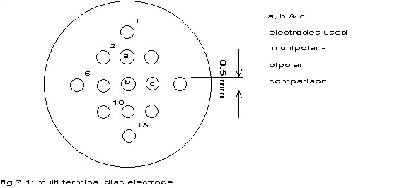
a, b & c: electrodes used in unipolar – bipolar comparison
If the electrodes, the amplifiers, the recording sites and the contacts between electrode and tissue are equal, the bipolar electrogram can be reconstructed from the unipolar electrograms. As explained in chapter III, par. 3 no good calibration was possible, but – assuming equalness and just a shift in time between the measured signals – the bipolar phase was calculated from the unipolar phases at the fibrillation frequency and compared with the actually measured bipolar phase. From the difference between these two a factor expressing the assumed unequal amplitudes was calculated for all three electrode sites. This factor could be calculated for one site in two different ways and so the accurateness of the method could be estimated. The results are put in table 7.3.
| minutes after start of VF | A{ab} | A{bc} | A{ac} | A{ab}/A{bc} | % | comments |
|---|---|---|---|---|---|---|
| 0 | 0.878 | 0.878 | 0.980 | 1.000 | -2 | See fig. 7.1 and appendix C. The last column expresses the percentage difference between column 4 and 5. The electrodes and amplifiers are stable, VF is unstable. |
| 2.3 | 0.848 | 0.823 | 1.029 | 1.030 | 0 | |
| 3.2 | 0.837 | 0.817 | 1.037 | 1.024 | 1 | |
| 126.0 | 0.902 | 0.819 | 1.049 | 1.101 | -5 | |
| 127.1 | 1.019 | 0.913 | 1.085 | 1.116 | -3 | |
| 128.4 | 1.094 | 0.975 | 1.102 | 1.122 | -2 | |
| 200.0 | 0.404 | 0.879 | 0.440 | 0.460 | -4 | |
| 201.1 | 1.257 | 0.158 | – | 7.956 | – | |
| 326.0 | 1.096 | 0.868 | 1.209 | 1.263 | -4 | |
| 327.1 | 1.057 | 0.871 | 1.194 | 1.214 | -2 | |
| 328.5 | 1.520 | 1.113 | 1.403 | 1.367 | 3 |
The amplification and filter settings of the amplifiers had not been changed during the experiment and the electrode had been fixed to the epicardium, so the differences seen in course of time likely reflect changes in the electrical behaviour of the myocardium at the recording sites. The last column clearly indicates the reliability of the methods used.
The rest of this chapter will be devoted to unipolar cardiac electrograms for the reasons given above.
3. Size of coherent areas
- The basic fibrillation frequency is the frequency with the highest peak in the autopowerspectrum.
- Two electrodes will be called coherent, if the coherency between their signals at the basic fibrillation frequency is so high that the critical value associated with this level is surpassed.
- An area will be called a coherent area if all electrodes within that area are coherent.
3.1 Largest coherent area
In order to get some idea about the largest size of coherent areas 6 unipolar epicardial electrodes have been stitched to the heart as indicated in fig. 7.2 and the intramural needle was put into the septum.
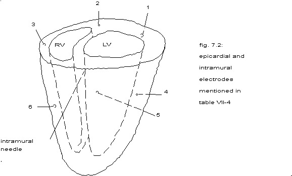
From table 7.4 one could conclude: during ventricular fibrillation apparently a coherent area can stretch sometimes all around the heart or be smaller than 2 mm.
| electrode | electrode | terminal | total | comment | |||||||
|---|---|---|---|---|---|---|---|---|---|---|---|
| 2 | 3 | 4 | 5 | 6 | 9 | 10 | 11 | 12 | |||
| 1 | 1 | – | 1 | – | 1 | – | 1 | – | – | 4 | |
| 2 | – | – | – | – | – | – | – | – | – | ||
| 3 | – | 1 | 1 | – | – | – | – | 2 | |||
| 4 | 1 | 1 | 4 | 3 | 2 | – | 11 | ||||
| 5 | 1 | 1 | – | 1 | – | 3 | |||||
| 6 | 1 | 1 | 1 | – | 3 | ||||||
| terminal | |||||||||||
| 9 | 4 | 3 | – | 7 | |||||||
| 10 | 4 | 3 | 7 | ||||||||
| 11 | 4 | 4 | |||||||||
| total | 1 | – | 1 | 2 | 4 | 6 | 9 | 11 | 7 | 41 | |
As the expected number of accidental coherencies within 41 pairs at the significance level of 0.001 is 0.41, all coherencies found can be considered as real.
3.2 Change in size of coherent area
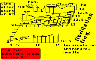
In the above figure the changes in size of coherent areas and in strength of coherency have been sketched for a particular experiment (dog # 28016) over a period of approximately 100 minutes. The numbers on the horizontal axis indicate the terminals on an intramural needle electrode in the septum, from which unipolar electrograms have been derived (see chapter III, par. 3 for more details). The basic fibrillation frequency remains stable between 12.5 and 13 Hz (the bandwidth is 0.5 Hz). At the start of ventricular fibrillation terminals 3 and 4 are not coherent with the other terminals; they exhibit a repetition frequency of 11.5 Hz.
3.3 Discussion
No explanation can be given for the fluctuations in strength of coherence. The size of coherent areas nor their position along the needle are constant and in the next chapter a model will be proposed that offers an explanation. From the fact that in this and several other experiments sometimes one terminal can be found incoherent with its neighbours, was concluded that the field contributing to the measured potentials of a terminal does not extend over more than 2 mm (the distance between the terminals). All experiments with the intramural electrode and the epicardial electrode showed that the size of coherent areas ranged from less than 2 mm to more than 24 mm.
4 Wavefront propagation in coherent areas
4.1 Introduction
If during ventricular fibrillation a wavefront travels around the heart in a fixed path, all areas of the heart fibrillate with the same frequency and with a fixed phase shift, i.e. all areas are coherent. If however a wavefront travels around the heart in an ever changing path, than also the phase difference between two electrode sites changes continuously. A coherency will be found if the phase does not change too much and a lot of the coherencies in table 7.4 could be explained in this way. The fact that not all of the intramural terminals are coherent – there always is a coherency over 2 mm, most of the time over 4 mm and never over 6 mm distance – must then be explained by assuming that this ‘path’ changes its course repeatedly even in a piece of tissue of 6 mm. On the other hand one must assume that at the same time this ‘path’ is constant over a large distance, as in a great number of cases a coherency has been found between electrode 4 and terminals on the intramural needle. Probably the conduction tissue plays a role, but the next paragraph makes the idea of conduction during ventricular fibrillation much more questionable and the next chapter offers a model that explains these features in an other way.
4.2 Travelling wavefronts
First of all will be discussed how the concept of travelling wavefronts leads also to paradoxical results. If two electrode sites (a,b) are very close together, the wavefront can be considered as a straight line crossing the line a-b at an angle .
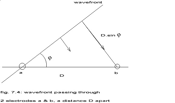
If v represents the actual velocity of the wavefront and D the distance between a and b, then the apparent velocity v’ between a and b is:
v’ = v / sin
A negative angle will lead to the same apparent velocity, so:
v’ = v / |sin |
If = �
then v’ = v.
If = 0 then v’ =
Of seven dogs all apparent velocities between adjacent unipolar terminals on the intramural needle or the epicardial electrode are shown in the form of a histogram in the next figure.
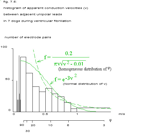
The few velocities lower than 0.1 m/s will for the moment be left out of the discussion. If the travelling wavefront concept during ventricular fibrillation is correct and if a constant and uniform velocity of propagation of that front is assumed, than that velocity during ventricular fibrillation is about 0.1 m/s. This figure is not too far away from the normal conduction velocity in the ventricle of 0.4 m/s as given in literature (Scher 1976). The second horizontal axis in fig. 7.5 indicates the angle the wavefront must make with the line between two electrodes to result in the apparent velocity of the first axis.
4.3 Velocities
The continuous line in fig. 7.5 indicates the best fitting Normal distribution, taking into account that although a negative velocity could be explained as belonging to a front travelling in a direction opposite to a front with a positive velocity, only positive velocities have been calculated. Anyhow, the apparent velocities do not follow a Normal distribution. If the wavefronts are assumed to hit the line between two electrodes from all directions, i.e. the angle (see fig. 7.4) is homogeneously distributed between – �
and �
, then the theoretical distribution of the apparent velocities can be derived as follows:
v’ = v / |sin |
F(v’) = P(V’ <= v’) = 2{P( >= arcsin(v/v’))} =
= 2{1-P( <= arcsin(v/v’))} = 2{1-(arcsin(v/v’)+�
)/
} =
= 1-(2.arcsin(v/v’))/ ; i.e. a Cauchy distribution
f(v’) = F'(v’) = 2v / ( v’
(v’�-v�))
For v=0.1 m/s this theoretical distribution density has been indicated with a broken line in fig. 7.5.
No systematic differences have been found between the 7 dogs, so the fact that the apparent velocities do not follow this theoretical density must be explained either by assuming a non-uniform conduction velocity over the ventricle or by rejecting the homogeneous distribution of , i.e. by assuming a preference for the wavefront to hit the line between two electrodes at small angles.
4.4 Travelling wavefront reconstruction
The latter possibility has been worked out in the next figure.
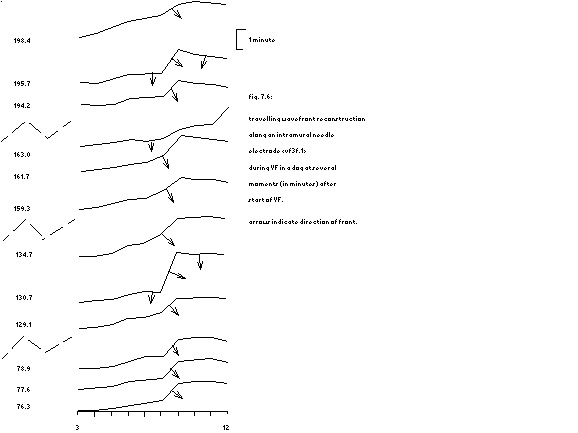
arrows indicate direction of front.
In the only case ( # 03037) where all unipolar terminals on the intramural needle remained coherent throughout the experiment, the angles of the wavefront with the needle have been estimated from the apparent velocities between the terminals, assuming a conduction velocity of 0.1 m/s. By connecting the lines representing these angles a kind of total travelling front has been reconstructed. The direction of the “front” has been indicated by arrows. Clearly the preference for small angles can be seen in this example and this could be accidental. The fact however that for all electrodes this preference exists, regardless of there position, makes the other assumption of a non-uniform velocity more plausible. Fig. 7.6 also indicates that in that case the conduction velocity not only is different over distances of about 2 mm, but also changes in time.
If one has to assume locally and temporally varying conduction velocities maybe it is easier to assume there is no conduction at all (see the next chapter). In the remainder of this paragraph some reasons will be given to reject the idea of conduction during ventricular fibrillation.
In table 7.3 is indicated that 201.1 minutes after the start of ventricular fibrillation not all phases could be estimated because of lack of coherency. That block of 20×2 seconds was analyzed in detail. Assuming orderly travelling wavefronts over small distances, 5 ms isochrones have been sketched between electrodes a, b and c (fig. 7.1 at intervals of 2 s.
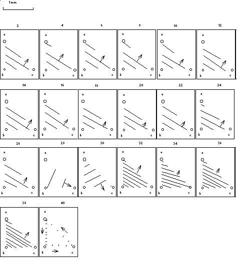
topnumbers indicate 2 s intervals
The first 26 seconds a rather regular ‘front’ seems to travel from b to a and c at a speed of circa 0.05 m/s; see the first 13 blocks in fig. 7.7. Suddenly the ‘speed’ increases to 0.1 m/s and the direction of the ‘front’ changes 90�; then the ‘speed’ returns to 0.05 m/s, thereafter the direction changes 90� back and the ‘front’ slows down to 0.02 m/s (the next 3 blocks in fig. 7.7). The next 3 episodes of 2 seconds the ‘front’ stays stable and then suddenly dissolves into a circular movement with a ‘speed’ varying between 0.025 and 0.05 m/s.
5 Phase and antiphase
5.1 Circular histograms
The estimated phase between all unipolar electrodes within the three coherency classes (table 7.5) has been displayed in a circular histogram. The radial distance corresponds to the number of phases in a particular angle class, the top corresponds to in-phase and the bottom to anti-phase. The strongly coherent electrodes are predominantly in-phase, but in the weakest coherency class also anti-phase relationships are present. In none of these groups a random distribution over all possible angles has been found.
| class | K� | circular histogram | |
|---|---|---|---|
| lower limit | upper limit | ||
| 1 | 0.2113 | 0.5322 | 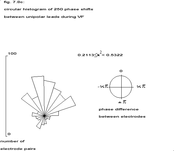 |
| 2 | 0.5322 | 0.8161 | 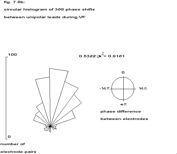 |
| 3 | 0.8161 | 1.0 | 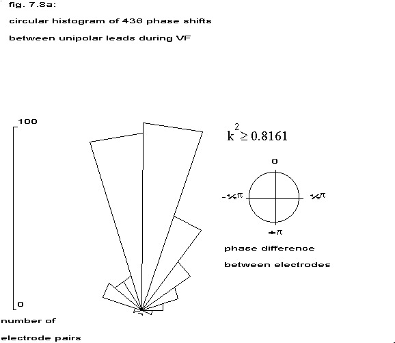 |
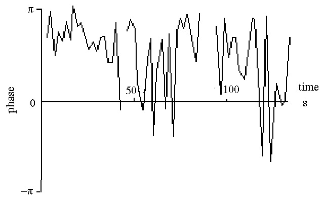
5.2 Instable phase shifts
An example of instable phase shifts is given in the next figure. Two intramural needles were put into the septum perpendicular to each other and the phase shifts at 11 Hz between the coherent bipolar leads were transformed into milliseconds delay or advance relative to the first pair of electrodes on needle A. The whole area spanned by the needles was coherent and the phases on needle A remained rather stable from 5 to 6.4 minutes after the start of ventricular fibrillation. The change of the fifth pair from 43 msec to -45 msec does not mean anything more than just a wobble around half a period delay or advance.
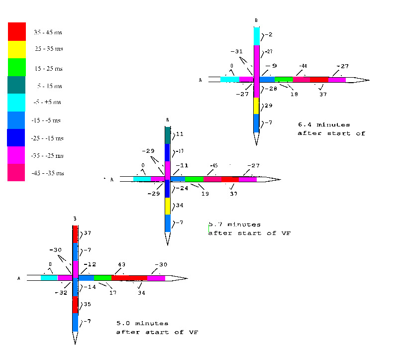
Some electrode pairs on needle B however show drastic changes in phase which are hard to reconcile with the concept of travelling wavefronts. The other stable phase shifts are even more difficult to explain within that concept.
As already stated in this paragraph “phase” means the cross phase spectral value at a certain frequency band averaged over 20 consecutive blocks of 2 seconds.
shift from anti-phase to in-phase
coherency block 10-12 in fig. 7.3
power spectra fig. 7.12
cross phase fig. 7.23
phase shift? fig. 7.14
action potential fig. 7.15
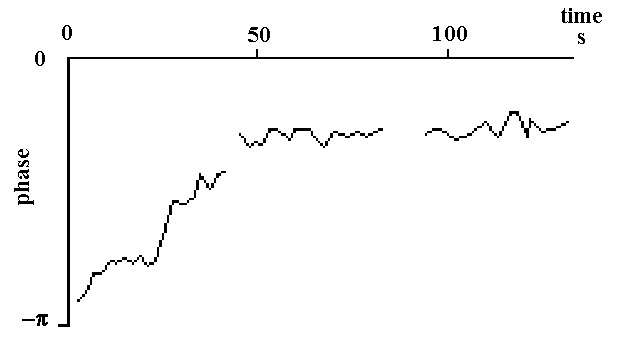
In fig. 7.10 is illustrated how the cross phase per such block at 12.5 Hz between two adjacent terminals on an intramural needle changes in course of time. At the start of the measurement (83.7 min. after the start of ventricular fibrillation, coherency block 10 of fig. 7.3) the two sites are in anti-phase, but gradually this changes to a constant much smaller phase difference. Not surprisingly this resulted for the first group of 20 blocks in a middle type of coherency and for the other two in a strong coherency. The averaged phases were resp. -0.63 p, -0.29 p and -0.26 p .
gradual loss of coherency
coherency block 10-12 in fig. 7.3
simultaneous coherency in fig. 7.10
Figure 7.11 illustrates the behaviour of this instantaneous phase if the coherency between two adjacent terminals is weak (group 1 and 2) or absent (group 3). These measurements came from the same needle at the same time as those of fig. 7.10.
5.3 Phase and form
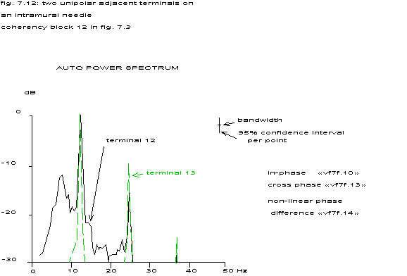
coherency block 12 in fig. 7.3
in-phase fig. 7.10
cross phase fig. 7.13
non-linear phase difference fig. 7.14
In the figure above the autopower spectra of two adjacent terminals (12 & 13 unipolar) on an intramural needle are shown directly after the start of ventricular fibrillation. (Dog # 28016, same as in fig. 7.3 and fig. 7.10. Both spectra contain clear sharp peaks at 12.5, 25 and 37.5 Hz plus a more or less clear peak at circa 6.25 Hz.
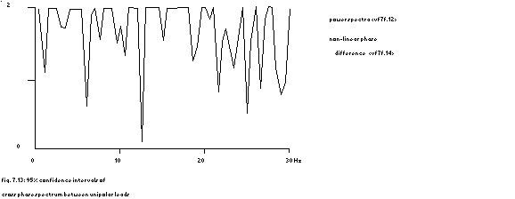
power spectra in fig. 7.12
non-linear phase difference fig. 7.14
The 95% confidence interval per frequency band is shown in the figure above and clearly is seen how the terminals are coherent at the frequencies mentioned and much less or not at all at other frequencies.
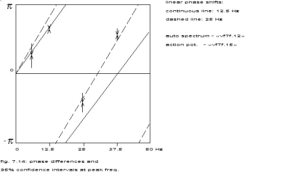
linear phase shifts:
continuous line: 12.5 Hz
dashed line: 25 Hz
auto spectrum in fig. 7.12
action potential in fig. 7.15
The actual averaged phase difference between the terminals has been drawn in fig. 7.14 for the frequencies 6, 12.5, 18.5, 25, 31 and 37.5 Hz. The vertical bars indicate the confidence intervals and the straight lines indicate the expected phase shifts if there is a simple time delay between the signals of terminal 12 and 13. The continuous line falls within the confidence interval of 12.5 Hz and the broken line within the interval of 25 Hz.
Both lines deviate strongly from the other confidence interval, so in this case the whole concept of a travelling wave has to be suspected. This has been indicated in the next figure maybe even more clearly.
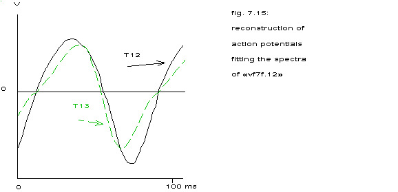
see the spectra in fig. 7.12
Here a reconstruction has been attempted like in chapter 4 of the extracellularly measured action potential giving rise to a spectrum as in figure 6.7. The curves have been aligned in such a way that they cross the zero level in at least one point simultaneously. The top of T13 clearly comes later than the top of T12, but then T13 advances in respect to T12, so it makes no sense to talk about a time shift as both curves are so much different.
5.4 Discussion
The previous figures just give an example how form differences in the complexes measured at adjacent electrode sites lead to cross phase spectra that cannot be interpreted in terms of time shifts. Most of the estimated power spectra differ in the relative heights of their peaks, so probably the phenomena displayed in fig. 7.6 and fig. 7.7 do not depend on time lags but on form changes.
6 Conclusion
The so called basic fibrillation frequency is explained in chapter VI, par. 4.2 as the result of two groups of cells active at half that frequency but in anti-phase. If there are changes in the contribution of one group to the potential of the electrode compared to the other group, then the phase also changes and the amount of ‘unequalness’ between two sites changes with it. This is in accordance with the behaviour of the model in chapter V, par. 4 and with the changes found in amplitude of the frequency peak at half the fibrillation frequency (fig. 4.12).
Some evidence has been given in this chapter that even at distances of 2 mm the amplitude and the form of the extracellularly measured action potential might differ so much, that the bipolar electrograms during ventricular fibrillation do not carry the same information as in the case of a regularly beating heart. The unipolar electrograms are of course comparable to those made in a beating heart, but the cross phase spectrum (and necessarily the crosscorrelation function ) is not only dependent upon eventual time lags between electrode sites but also upon those form changes. Moreover, the strong predominance of small phase differences – specially in the strongly coherent areas independent of electrode distance – makes the assumption of conducted wavefronts during ventricular fibrillation highly improbable.