1 Introduction
A repetition frequency in the range of 4.5 to 6.5 Hz (equivalent to 270 to 390 beats per minute or an interval range of 150 to 220 ms) fits the known physiological properties of the myocardial cells of the dog much better than the twice higher frequency found in signal analysis, see chapter IV, par. 4. In the previous chapter (par. 3.5) was shown the tendency of the modelcells to get organized into two groups of more or less synchronized cells. In this chapter the output of the topological model will be treated as an electrogram during fibrillation in order to throw some light upon the results of chapter 4.
2 Simulated potentials
The measurable electrical activity of the model was simulated by assuming that the membrane potential could be described by the sum of 2 integrals of Gauss-curves:
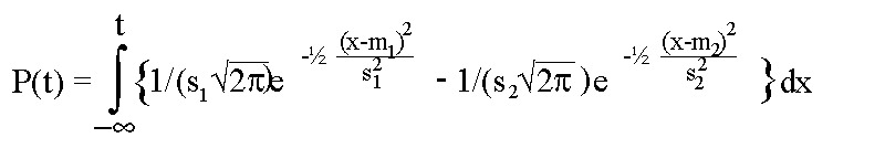
where
- P(t) stands for the membrane potential at time t after activation,
- m1, s1 for the steepness of the upstroke and
- m2 and s2 for the steepness of the downstroke of the membrane action potential.
The length of the action potential is determined by m1+m2.
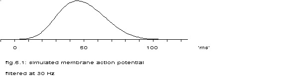
P(t) is drawn for m1=30, s1=10, m2=65 and s2=15.
The extracellular action potential after stimulation is reasonably well approximated by the second derivative of the membrane potential in course of time, (Scher 1979). Thus:
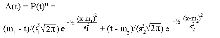
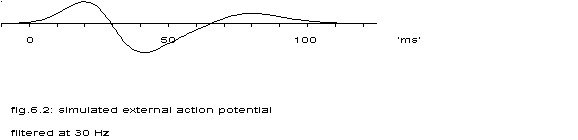
A(t) with m1=30, s1=10, m2=65 and s2=15.
These formula’s were used to transform the output of the topological model into something that appeared like an electrogram, see the next figure for an example.
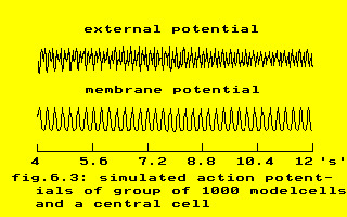
The apparently twice higher frequency of the conglomerate of 1000 model cells – compared to the ‘membrane potential’ of the central cell – is clearly seen. (The model is described in chapter V, par. 3.5).
3 Histogram
The amplitude histogram of the ‘membrane potential’ of the central model cell is depicted in the next figure.
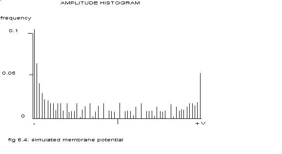
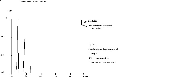
see fig. 6.3
power spectrum in fig. 6.8
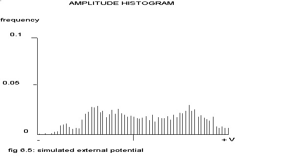
Such a histogram is typical for a (almost) sinusoidal distribution. The histogram of the ‘extracellular electrogram’ of the above mentioned conglomerate of 1000 cells is shown in the next figure.
see fig. 6.3
power spectrum in fig. 6.9
This histogram is almost identical to that in fig4.7 in chapter IV. Maybe the most interesting type of histogram is this two-peaked form. If the signal from one electrode can be considered as the sum of n independent sinusoidal distributions, other types of histograms will be found and according to the central limit theorem in statistics even a normal distribution when the number n grows to infinite. To see how fast the sum of such a histogram would look like a normal distribution, the amplitude histogram of 1000 pseudo-random drawings from such distributions has been calculated.
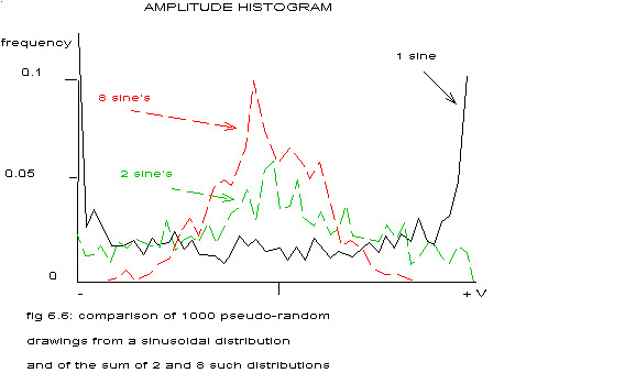
In the figure above the results are depicted for the sinusoidal distribution and the sum of 2 or 8 independent sinusoidal distributions. If the number n equals 8 the amplitude histogram is already unimodal symmetric, so instead of assuming different types of ventricular fibrillation in different parts of the same heart, one could also – restricting oneself to histogram analysis – assume one type of ventricular fibrillation giving rise to a sinusoidal signal in such small, independent islands of heart tissue, that in most cases the electrodes used will record the summed electrical activity of several of these islands.
4 Power spectrum
4.1 Peaks at regular intervals
Repetition of a function ad infinitum at regular intervals t removes all of the Fourier transform except delta function samples at f=+n/t (n=0,+1,+2,…). The derivation of these results is seen simply if the process of repetition is regarded as the convolution of a function with an infinite set of regularly spaced delta functions (Champeney 1973). The theoretical power spectrum of A(t) (see par. 1) plus its convolution with a train of delta functions is sketched in the next figure.
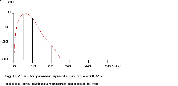
added are deltafunctions spaced 5 Hz
see fig. 6.2
In other words: the Fourier transform of a repeated function is equal to zero except at the repetition frequency and its higher harmonics, where the transform equals the original Fourier transform of that function. The power spectra of the ‘potentials’ shown in fig. 6.3 are depicted in the next 2 figures.
see fig. 6.3
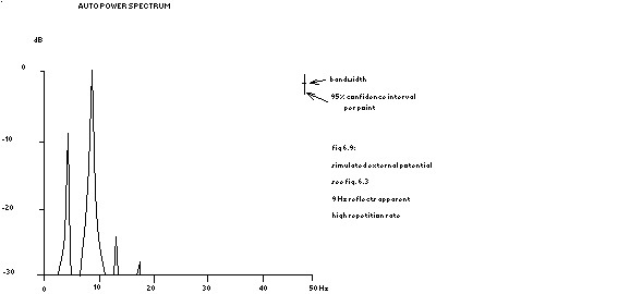
9 Hz reflects apparent high repetition rate
see fig. 6.3
The horizontal axes are redrawn in such a way, that one timestep stands for 2 msec’s.
4.2 Subharmonics and alternans
The spectrum of the total activity would lead to the conclusion of a repetition frequency of ventricular fibrillation of 9 Hz like in our previous publications (Herbschleb 1979, Herbschleb 1980a and Herbschleb 1980b). Analysis of individual cells (the central cell is shown as an example) however shows that the cells have a repetition frequency of 4.5 Hz. The two groups of model cells are not quite equal in size, so a clear alternans in amplitude is present. As will be proven in appendix E, this means that the low repetition rate of the individual cells is present in the spectrum as a low peak at a frequency half of the overall repetition frequency. In chapter IV – par. 4.1 – has already been mentioned that 25% of the auto power spectra during ventricular fibrillation exhibit this low frequency peak. An example of a subharmonic peak has already been given in fig. 4.25 and another one is given in the next figure.
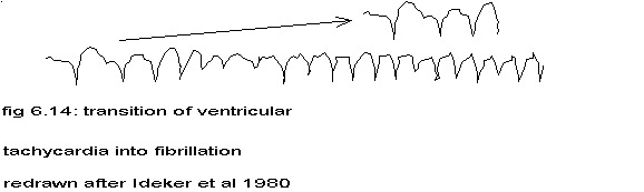
Another indication is seen in fig. 11.8 and fig. 11.9 showing the cardiogram of an intramural needle electrode (unipolar) during the transition from a very fast ventricular rhythm (stimulation by electrical pulses of 5 msec duration at 20 msec intervals) to ventricular fibrillation. Not only is the repetiton rate during ventricular fibrillation immediately twice the rate during regular contractions, but clearly the fibrillation waves alternate in height. The same phenomenon is present in figure 11 of Ideker et al (Ideker 1980) and in figure 2A of Sano et al (Sano 1958) – see figures 6.14 and 6.13 – and the doubling of frequency in figure 3 of Josephson et al (Josephson 1980) – see fig. 6.15 – and less clear in figure 8 of Vanremoortene (Vanremoortene 1968). None of these authors mentions these features of their figures. In chapter IX more evidence will be presented to support the claim, that ventricular fibrillation is a tachycardia with a splitting of the phases of the cells in 2 opposite groups.
5 Regularity
If the repetition is not exactly regular, but some irregularity like e.g. a regular modulation of the intervals is present, the delta functions mentioned will be accompanied by sidebands, which will result in practical signal analysis in broadening of the peaks. The more irregular the repetition, the less peaks are discernible. As shown in appendix E one could use the figures of that chapter as a kind of nomogram to express the regularity of ventricular fibrillation as the coefficient of variation – cv=s/m – (standard deviation divided by the mean) of the repetition interval. Assuming a normal distribution of the intervals, 95 % of the intervals will lie in between m-1.96·s and m+1.96·s; in terms of coefficient of variation: 95 % lies in between m(1-1.96·cv) and m(1+1.96·cv).
| figures | cv | frequency | m | 95 % interval |
|---|---|---|---|---|
| fig. 4.12 | 0.025 | 11.5 Hz | 87 ms | 79 – 95 ms |
| fig. 4.13 | 0.156 | 10.5 Hz | 95 ms | 66 – 124 ms |
| fig. 4.14 | 0.25 | 10.5 Hz | 95 ms | 48 – 142 ms |
| fig. 4.25 | 0.075 | 11.5 Hz | 87 ms | 74 – 100 ms |
| fig. 4.26 | 0.125 | 10.5 Hz | 95 ms | 73 – 118 ms |
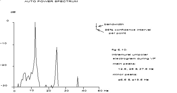
| fig. 6.10 | 0.025 | 12.5 Hz | 80 ms | 76 – 84 ms |
tabel 6.1: Classification of spectra in this study, using the width of the second spectral peak at -20 dB
6 Reconstructed action potential
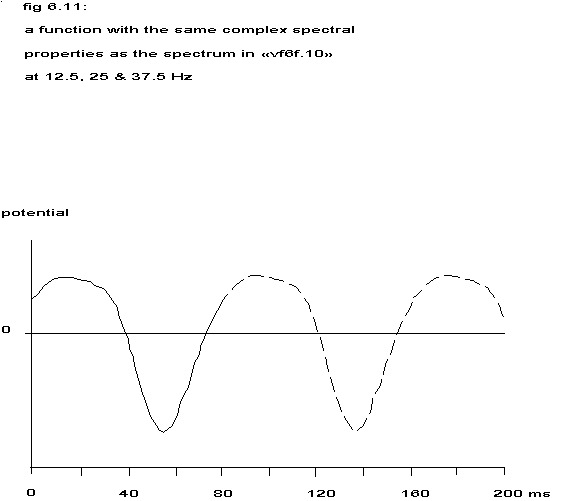
The spectrum in fig. 6.10 contains very sharp peaks at the frequencies 12.5, 25 and 37.5 Hz and less predominant peaks at 6.0 – 6.5, 18.5 – 19.0 and 31.0 Hz. Assuming a completely regular repetition (cv < 0.025, see previous paragraph) and considering the estimated spectral values at 12.5, 25 and 37.5 Hz as the best estimation of the height of the delta functions mentioned earlier, one could reconstruct an idealized function with such a spectrum by inverse Fourier transformation.
Taking into account the spectral values at the half frequencies, inverse Fourier transformation yields a function like in the next figure.
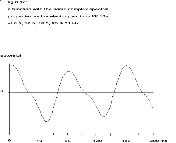
This function differs in shape from the one in fig. 6.11 and also displays a clear alternans. The spectrum of fig. 6.10 belongs to an unipolar, intramural electrogram from an electrode with a surface of 1 square mm. Such an electrode collects the electrical output of a great number of cells and if all these cells fire at random the result is something akin to white noise. If the cells that contribute most to the potential field of the electrode are in synchrony and fire regularly, a spectrum with sharp peaks at the repetition frequency and its higher harmonics will arise. Should there however be two equal groups of cells firing very regularly in synchrony, but with half a repetition period shift between the two groups, then the odd peaks would disappear from the spectrum, suggesting a twice higher repetition frequency than really present; see appendix E. If these two groups are not exactly equal, whether in size or contribution to the potential field of the electrode, the odd frequencies will still be present in a diminished form like in fig. 6.10.
The height of the even peaks is equal to the sum of the corresponding spectral values for the separate groups and the height of the odd peaks is equal to the difference of the corresponding spectral values. If one assumes that the spectra of both groups do not differ in shape and that the recorded extracellular waveform is proportional to the second temporal derivative of the membrane action potential (Scher 1979), then from the complex spectrum a reconstruction of the membrane action potential would be feasible. This reconstruction with the help of the complex spectrum belonging to the power spectrum of fig. 6.10 is sketched in the next figure.
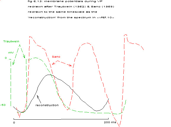
Redrawn after Trautwein 1952 & Sano 1958
Trautwein and Zink published repetition rates of single heart cells in frogs, dogs and cats (Trautwein 1952). Contrary to Sano 1958 their recorded membrane potentials became completely repolarized between contractions and the repetition frequency during ventricular fibrillation was slightly higher than the highest normal beating rate (250 beats/min versus 200 beats/min). Reasonably normal action potentials during ventricular fibrillation were also reported by Hoffman and Suckling (Hoffman 1954).
First of all nothing more has been stated than: if the above mentioned function is repeated regularly at intervals of 160 ms (375 pm) and a second identical function is formed with a 80 ms shift and the sum is formed of proper weight factors times the temporal second derivatives of these two repeated functions, then this sum will have a power spectrum like the one in fig. 6.10, but many other functions will yield the same spectrum, as only information of the frequency components of 6.25, 12.5, 18.75, 25, 31.25 and 37.5 Hz is available.
Furthermore, if one wishes to compare the reconstruction to the actual action potentials as reported in the literature fig. 6.13, one should keep in mind that the original signal had been filtered at 30 Hz.
7 Anatomy
In this paragraph a lot of loosely connected remarks are presented, that throw some light on the reasoning behind the model of chapter V.
7.1 Nexus
Sperelakis and Hoshiko (Sperelakis 1960) supported the theory of junctional transition between myocardial cells by showing there are no low resistance pathways between cells. By phase-contrast microscopy was shown that in living tissue the intercalated disks were clearly seen and that they formed no fixation artifact (Yokoyama 1961). Moreover they observed how these disks formed a definite partition between a segment of the fiber which survived and contracted and an adjoining portion which failed to contract.
The idea that one myocardial cell can excite another, if there are enough nexuses between them, comes from the observation of Goshima 1975 in tissue cultures that one single myocardial cell will synchronize another, even if the current flows via a non-excitable cell in between.
7.2 Repetition frequency
From theoretical studies (Winfree 1980) and experimental work (Jongsma 1975) it is known that an aggregate of coupled periodically active elements can beat (much) faster than the isolated elements. All myocardial cells are thus supposed to be potential pacemakers; Goshima 1975, who reports that 70% of single fetal myocardial cells in culture is spontaneously active.
Although thus theoretically an increase in spontaneous activity from 20- 40 b.p.m. (3000-1500 ms) in complete heart block to 6.5 Hz (154 ms) during ventricular fibrillation in human patients cannot be excluded, the sudden frequency doubling from ventricular tachycardia (150-220 b.p.m.; 400-273 ms) into fibrillation is not explained be these models.
7.3 Neighbouring cells
In fig. 5.6 one can clearly see how neighbouring ‘cells’ are in opposite phases. Although this might seem impossible in an actual heart to physiologists who more or less tacitly assume a syncytial heart tissue, Imchanitzky indicated already in 1905 and 1906 that adjacent cells in the myocardium during ventricular fibrillation could be in quite different states, i.e.: one was fully contracted and its neighbour relaxed ( Imchanitzky 1905 and Imchanitzky 1906). The model thus exhibits the focal reexcitation phenomenon as defined by Han: “due to the flow of current between adjacent fibers that are repolarized at grossly disparate times.” (Han 1971).
7.4 Size considerations
An aggregate of 10 by 10 by 10 cells of the dog myocard will have dimensions of circa 1.0 by 0.1 by 0.1 mm. Such a small piece of tissue would stop fibrillation immediately or after several seconds, see Garrey 1914, so the instability of the model is not surprising. All cells in such a group are supposed to have the same characteristics, as the tight electrotonic coupling prevents significant differences in e.g. action potential duration, see Mendez 1969.
8 Some mathematical remarks
No attempt was made to describe the action potentials and membrane coupling in terms of the Hodgkin-Huxley equations, as it would cost too much to resolve them simultaneously for 1000 cells. Moreover some justification for the methods of chapter IV comes from the statement by DeHaan and DeFelice (DeHaan 1978): “The magnitude and kinetics of recorded electrical events may reflect tissue geometry more than the characteristics of the cell membranes”.
9 Conclusion
Keeping all this in mind the results of chapter IV could be explained as being caused by measuring during ventricular fibrillation a fairly regular electrical phenomenon or the sum of a number of such independent phenomena. This phenomenon consists out of action potentials of myocardial cells, organized in 2 interwoven groups that constantly activate each other.
10 P.S.
After completion of the text I added 2 more examples of frequency-doubling. See par. 4.2 for an explanation.
redrawn after fig. 11 in Ideker 1980
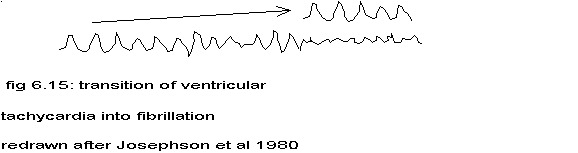
redrawn after Josephson 1980