V. A LOCAL, OSCILLATING MODEL

the basic unit for ventricular fibrillation

1 Introduction

As discussed already in chapter 2 those authors, who proposed models of ventricular fibrillation, considered atrial fibrillation as the same type of electrophysiological phenomenon as ventricular fibrillation, for the understandable motive that atrial fibrillation is not a lethal arrhythmia and thus much easier to investigate than ventricular fibrillation. See: Moe 1964, Ritsema van Eck 1972, Foy 1974 and Allessie 1977. Moreover they created one-level models consisting of elements without known anatomical and physiological properties. With differences between atrial fibrillation and ventricular fibrillation as indicated in the previous chapter, the two-dimensional sheet models of Moe, Foy and Allessie look rather unrealistic for the ventricle, the spiraling waves in sheets without anatomical obstacles as described by Foy and Allessie are contradicted for ventricular fibrillation in this study chapter VII and the strong irregularity during selfsustained activity in the three-dimensional model of Ritsema van Eck is not in accordance with the results in chapter IV.

In this study an attempt is made to describe ventricular fibrillation with a two-level model. The first, lower level will be discussed in this chapter and in the next as self-sustained activity within a relatively small group of interconnected cells, based upon the results of the single channel analysis of chapter 4. The second, higher level (chapter VIII & chapter IX ) describes the interactions between these groups, based upon the multi channel analysis of chapter 7. The availability of large, digital computers created the possibility of modelling the electrical activity within the myocardium as the result of interactions between individual cells, instead of approximating this activity by field equations and approximating the solution of these equations by a digital computer. The models intended are thus discrete (contrary to analog) and automatic (contrary to input-output systems), as the myocardium does not react to normal, physiological stimuli during ventricular fibrillation. A “discrete automaton” or simply “automaton” designates a model which has the following features:

1. at each of the discrete instants of time t1,t2,…,tm input values x1,x2,…,xm each of which assume a number of fixed values from the input set X, are applied on the input of the model;
2. on the output of the model n output values y1,y2,…,yn can be observed, each of which can assume any number of fixed values from the output set Y;
3. at each instant of time the model can be in one of the states z1,z2,…,zN;
4. the state of the model at each instant of time is determined by the input value x at this time and the state z in the preceding instant of time;
5. the model realizes the transformation of the situation at the input x={x1,x2,…,xm} into the situation at the output y={y1,y2,…,yn} depending on its state in the preceding instant of time.

See Lerner 1972.

A mathematically more rigorous definition of an automaton would be (Barto 1975): an automaton (or sequential machine) is a quintuple M=

1. X is a non-empty set of input values;
2. Q is a non-empty set of states;
3. Y is a non-empty set of output values;
4. f: Q . X -> Q is the transition function and
5. g: Q -> Y is the output function.

M is a finite automaton when X,Q and Y are finite sets.

Such a finite state machine is a theoretical device with a finite number of states, one and only one of which it must be in at any given time. A cell is one of the infinity of finite-state machines in a cellular space. A polyautomaton is a multitude of interconected automata operating in parallel to form a larger automaton, a macroautomaton formed of microautomata, an interconnection of cells.

Each cell gets its input from the outputs of a finite set of cells, forming its input neighbourhood, and possibly from an external source. Each cell computes its output at each tick of the clock, and the output is distributed to its output neighbourhood, a finite set of cells, and possibly to an external receiver. In this study it is assumed that all cells of a given polyautomaton are identical – the polyautomaton is monogeneous. Similarly it is assumed here that any polyautomaton is input-output symmetric, i.e. the connections between cells serve both as input and as output channel. In this study a cell does not belong to its own neighbourhood, i.e. a cell’s output does not influence its state at the next time step. See Smith 1976.

This description leads to the following extension of the definitions given above for the cells:

6. S is a non-empty finite set of identical cells of magnitude M;
7. E is the (infinite) complement of S in cellular space, called the environment of S;
8. N is a non-empty set of connector values;
9. C is a M.M matrix of connector values; a zero value indicates no connection.

Chosen for this study:

• x, q and y designate elements belonging to X, Q and Y respectively,
• s(i), s(j) designate elements belonging to S,
• c(i,j) indicates the connector value (from matrix C) between s(i) and s(j).
• The particular x, q and y values of a cell are indicated by parenthesized characters.
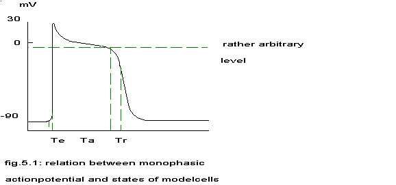
• The state q is an ordered set {qa,qm}, with qa indicating the actual state the cell is in and qm a memorized state.

1. x(i)= c(i,j.y(j))
2. qa=0 : quiescens
   0 < qa <= Te : excitation
   Te < qa <= Ta : activity
   Ta < qa <= Tr : absolute refractoriness
   Tr < qa <= Tm : relative refractoriness
   qa > Tm : qa = Te+1
   Te, Ta, Tr and Tm are model dependent parameters, finite, positive integers indicating time steps; Te=0 is permissible; a very large value of Tm blocks automaticity of the elements; the names of the different states have been phrased in physiological terms for ease of discussion;
3. Y={0,1}
   • for qa = 0
     • f{( 0, 0),x} = 0,0, if x < d(0,x)
     • f{(0,0),x} = 1,1 if x => d(0,x)
   • for 0 < qa < Te: f{(qa,qm),x} = qa+1,qm+1
   • for qa = Te
     • f{(Te,qm),x} = 0,0 if x < d(qm,x)
     • f{(Te,qm),x} = Te+1,0 if x => d(qm,x)
   • for Te < qa <= Tr: f{(qa, 0),x} = qa+1,0
   • for Tr < qa <= Tm
     • f{(qa,qm),x} = qa+1,h(qm,x) if x < d(qm,x)
     • f{(qa,qm),x} = 1,0 if x => d(qm,x)
   • for qa = Tm: f{(qa,qm),x} = Te+1,0
   h(qm,x) and d(qm,x) are model dependent functions;
   • g(qa,qm) = 1 if Te < qa < Ta
   • g(qa,qm) = 0 otherwise
4. M = 512 or 1000, 3-dimensional arrays of 8.8.8 or 10.10.10 cells the number was limited by available computer resources
5. the environment may or may not be connected to (a subset of) S
6. N is a finite set of integers
7. C consists of finite integers

Implicit in the description above is that x, y, qa and c(i,j) are finite integers. The state qm is real valued, but h(qm,x) will be chosen in such a way, that the number of memorized states per realization is finite. So the polyautomata described in this chapter are finite, uniform, deterministic, Moore-type (discrete time steps with a unit delay between an input and the associated output), autonomous or non-autonomous and static.

Clearly, h(qm,x), C and the begin condition of C remain to be specified for a particular model. In general the evolution of these systems is computationally irreducible to a more simple mathematical formula. Moreover, undecidable problems can arise in the mathematical analysis of such systems (Wolfram 1984). First an attempt has been made to study these models of ventricular fibrillation by lumping all elements together and look for the averaged, overall behaviour. The unsatisfactory results led to mathematical models that allowed for the study of individual elements.

2 Lumped models

2.1 introduction

The term “lumped model” is used to designate that class of mathematical models, that describe the overall behaviour of a system, without being able to simulate the behaviour of the individual elements. Wiener and Rosenblueth were the first to attempt to describe atrial fibrillation in this way as a special case of self-sustained activity in networks of interconnected excitable elements. (Wiener 1946). Their main assumption was that an element stayed only for an instant in the active state, which implies that the refractory state lasts much longer than the active state. This looks more representative for neuronal networks than for cardiac muscle cells and in that area a lot of work has been done; see Griffith 1971 for an introduction and review.

Several of these models have been described.See Bess 1970, Accardi 1972, Anninos 1972 and Burattini 1972. All agree upon the ease with which the networks show reverberations or periodical self-sustained activity.

2.2 model L1

variable	value
Te	0
Ta	1
Tr	3, 4 or 6
Tm	65000
h(qm,x)	1
C	c(i,j) = 0 except for 10 “randomly” chosen j’s = i, in such a way that the whole network is connected;
M	1000
begin condition of Q:	begin condition: q(i) = 0,0 except for a number of randomly chosen cells

In model L1 all cells possess a fixed number of connections with the other cells in the network, all cells have the same probability of being connected with each other and if a cell is connected to an active cell that cell also becomes active. The next step of simulated time the cell is no longer active, but refractory for a fixed number of time steps. Thereafter the cell becomes resting until stimulated. In a sufficiently large network the number of cells that become active may be supposed to be equal to the number of resting cells times the probability that at least one of the connections is active, regarding the total amount of activity at that moment in the network.

The model is started by introducing a certain percentage of activity into the network. A too low or too high percentage of activity does not elicit continuous activity, but the exact borders between persistent activity and transient activity have not been determined. The periodicity is equal to Tr. The reader can verify this easily by changing the parameters of the model LumpedL1. Whether the probability of becoming active is used in a deterministic way to get the actual number of active cells or stochastically by drawing that number from a binomial distribution did not make much difference, so the above mentioned model uses the expectation.

The assumptions in those models are too unrealistic to use these results for anything else than to show that a network of interconnected excitable elements easily exhibits periodical activity, even if the elements themselves do not show periodical activity. For an extensive, mathematical treatment of networks of logical neurones, see Holden 1976.

2.3 model L2

More realistic models to describe ventricular fibrillation were found in the field of epidemics (Waltman 1974); see chapter VI for a discussion on the interpretation.

Based upon the ideas of Waltman a model has been built using a modification of the simulation program Block CSMP of the IBM 1130.

  Te    4
  Ta   124

               F
  Tr   148 (K�M + Ta)
  Tm  65000
  M   1000
  h(qm,x) = qm+1

                             F
  d(qm,x) = exp((ln (qm + K�M  ) - ln K)/F) with K=90 and F=-0.19

Specially built delay lines were needed for the states: “excitation”, “activity” and “refractoriness”. The first three states had fixed delays of resp. 4, 120 and 24 msec, the last state had a variable delay depending on the overall activity, a maximal refractory period K and a ‘influence factor’ F (F <= 0). These times and factors were based partly upon the pictures published by several authors (Sano 1958, Krinsky 1973, Rushmer 1976, Cranefield 1975) and partly upon preliminary experiments with the CSMP model to find a stable continuous activity pattern. The relationship with the monophasic actionpotential is sketched in the next figure.

The normally quiescent model was brought to activity by gradually bringing a fraction of 0.0135 of the total population of 1000 cells into the active state every timestep during 74 timesteps of 2 msec’s. The rationale behind this is that it seems very unlikely that myocardial cells will have exactly the same refractory period and that stimulation of the heart with the high frequency of 50 Hz will bring all cells in a different phase in their cycle of stimulated activity. Zipes stated: “If the degree of electrical asynchrony is sufficiently great, then simply increasing the ventricular rate beyond the ability of all myocardial elements to follow in a uniform fashion will begin fibrillation.” (Zipes 1975) No stimulus whatsoever has been given after the first 148 msec. The reader can study this model in LumpedL2. In order to compare the output of this model with the experimental results every 20 simulated msec’s the value of the filtered first derivative of total activity was written to magnetic tape and analyzed in the same way as the recorded signals during ventricular fibrillation. The first derivative was chosen reasoning that an external electrode would measure a change in membrane potential rather than the spatial integral of all membrane potentials. The results of signal analysis are shown in

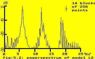
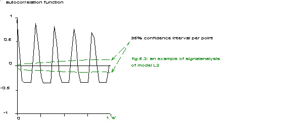
fig.5.3: an example of signal analysis of model L2

There is a clear resemblance to the results shown in chapter 4 up to the typical asymmetry of the autocorrelation function, however the main repetition rate is 6.25 Hz (equivalent to 160 ms) and definitely not 12.5 Hz.
The main drawbacks of this model are:

1. the absence of frequency doubling;
2. the fate of individual cells can not be followed;
3. no spatial organization can be introduced.

Or to paraphrase Scott on statistical neurodynamics: no difference will be found between a network with 1% of its cells becoming active a maximum rate and a network where all cells become active at 1% of the maximum rate. (Scott 1977). Its advantage was the demonstration that a simple network of inter-connected excitable (but not periodical) elements exhibited continuous, periodical activity, like the ring of hourglasses described by Winfree 1980.

3 A topological model

The above mentioned models all implied a repetition frequency of the individual elements (cells?) equal to the frequency of the aggregate. In dogs we found a fibrillation frequency of circa 12 Hz, roughly twice higher than the maximum rate of 300 heartbeats per minute in Beagles, ( Young 1961). The fact that the repetition period of the aggregate was always slightly longer than the sum of the periods of the three states (in the case of excluded enviromental influence on the length of the refractory period) of the constituent elements, plus the statement of Kermack and McKendrick (see Diekman 1978, pag. 54) that some elements in a population will escape an epidemic, hints at the possibility that at least some of the elements have a slower repetition frequency than the aggregate. In general a lumped model does not always exhibit the same behaviour as the base model (see Aggarwal 1975). So the need arose to construct a model consisting of discrete coupled elements, with the same characteristics as the cells in the preceding paragraph.

The known models that describe activity during ventricular fibrillation in terms of coupled elements, do not mean myocardial cells as elements, but – implicitly or explicitly assuming a myocardial syncytium – their elements are needed to discretisize otherwise intractable field equations. See e.g. van Capelle 1980, Foy 1974, Moe 1964, Ritsema van Eck 1972 and Mitchell 1992). At the microscopic level however, the assumption of a syncytium does not work very well, see Spach 1983. In this chapter however the “cells” of the cellular automaton are intended as models of real myocardial cells.

A general theoretical frame to analyze the behaviour of coupled, excitable, non-periodic elements is given by Winfree 1980. Practical considerations like available computer time and memory led to the construction of a model consisting of a three-dimensional array of 1000 cells (10�10�10). The essay of Fozzard 1979 on the conduction of the action potential in the heart establishes the anatomical feature called gap junction or nexus as the correlate for the electrical coupling between cells. The more nexuses, the stronger the coupling, see Plonsey 1974, Kensler 1977, Mann 1977, De Mello 1980, De Mello 1982a and De Mello 1982b. Based upon the anatomical data of Sommer and Johnson (Johnson 1967, Sommer 1979) the number of nexuses between cells was drawn from a binomial distribution, with a probability P and a size of 70. Tissue anisotropy and variation in junctions are sufficient for the necessary spatial variation; the assumption of variation in membrane properties is not necessary (Spach 1983). The cells are considered symmetrical and elongated in the X-direction; they have their nexuses only in the intercalated disks with a strong preference for the X-direction according to the following table:

p	z-1	z	z+1	illustration
y-1	0.02	0.04	0.02	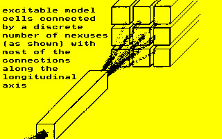Afbeelding ontbreekt
y	0.04	0.26	0.04
y+1	0.02	0.04	0.02

Table 5.1: probability used for the number of nexuses between a cell with coordinates x, y, z and its neighbours at coordinates x+1 or x-1, y-1 or y or y+1, z-1 or z or z+1

The total number of cellconnections thus amounts to 18 and the mean number of nexuses is 70 with a standard deviation of 7.7.

To resolve the problem of the border (a hypertorus was not considered an appropriate model) all 488 bordercells were connected to extra cells in a shell around the threedimensional structure. This shell could either be quiescent or be subjected to different types of activity to simulate the influence of the surrounding tissue on the simulated block. This random structure of cellconnections was created once and stored in a file for future parameter studies. The discrete timesteps in the simulations were supposed to represent 2 ms. In all cases the activity was started by distributing the cells, as uniformly as possible, random over the total number of timesteps in the states or phases of the activity cycle. The type of activity and its stability were investigated for the following models:

3.1 no input integration, fixed refractory period

   f{(Te,qm),x} = Te+1,0

   Te        2
   Ta       62
   Tr       82
   Tm    65000

   M      1000
   h(qm,x) = qm+1
   d(qm,x) = D

In words: If the number (x) of active nexuses (i.e. the number of connections with neighbour cells in the active state) of a quiescent or relative refractory cell exceeds the threshold (D), this cell enters the excited state; after 2 steps this cell enters the active state, becomes refractory 62 steps after excitation and quiescent again after 82 steps.

At threshold values (D) of 1, 5, 10, 15, 20 or 30 all cells were very regularly active with a repetition period of 164 steps; the total simulated period was 1000 steps. At the thresholds of 15, 20 and 30 a slight variation in the total number of active cells occurred, but of a random character. The output of the aggregate as a whole was somewhat noisy, but no periodicity became apparent. Raising the threshold to 35 extinguished activity within 328 steps; cells became active at irregular intervals.

3.2 input integration, fixed refractory period

The behaviour of real excitable cells, that only become active after stimulation during a certain time period, was simulated in the following way: an excited cell will enter the active state only if its number of active nexuses after Te steps still exceeds the threshold.

       f{(Te,qm),x} =    0,0         if x < d(qm,x)
                    = Te+1,0         if x >= d(qm,x)

The other parameters were not changed and the model behaved at thresholds of 30 and 31 just as above. At threshold 32 the total activity diminished slowly during the 1000 simulation steps and the cells fired less regular. At threshold 33 all activity ceased after 888 steps and at 35 after 425 steps; the firing pattern was totally irregular. Although the aggregate showed no periodicity in its stable activity at thresholds 30 or 31, the number of cells that became active at each timestep ranged from 7 to 17 with an average of 12.

The 1000 cells of the model could not be uniformly distributed over the 82 possible phases at the start of simulation. To check the possibility that the observed variation was caused by the initial irregularity, the lengths of the periods were changed to 3, 76 and 100, so the proportions did not change too much and the 1000 cells could now be distributed over 100 phases. At a threshold of 30 this model showed an exact repetition period of 100 steps in individual cells, but the overall variation in number of cells that became active was still there. This variation was too irregular to impose a periodicity on the whole model and was caused by the fact, that after the initial activation some cells cannot become excited and/or active as not enough of their neighbours are active. After a few cycles however all cells in this network ran as fast as they can, although the threshold of 30 is higher than the average number of connections between the most strongly connected cells: 0.26�70 = 18.2.

3.3 integrated input, relative refractory period

A certain periodicity is measurable outside the model only if the constituent cells should synchronize in such a way, that large groups of them would have the same phase. The check at the end of the excited state is apparently not enough for this purpose. At this stage of model building the quiescent state was replaced by the relative refractory state.

      for Tr < qa < Tm: f{(qa,qm),x} = qa+1,h(qm,x)   if x < d(qm,x)
                                     =    1,0         if x >= d(qm,x)
      h(qm,x) = qm + 1 - F�x/N ( 0 <= F < 1 )
      d(qm,x) = exp(-0.22(qm - 21)) + D
      N = total number of nexuses of a cell

In words: Cells will enter this state from the absolute refractory state and leave it for the excited state if their total number of active nexuses exceeds the threshold. Accomodation (Katz 1966) of the cell to sub-threshold stimuli is arrived at by subtracting from qm the number of active nexuses divided by N times a factor (F). The influence of this factor is sketched in the next table.

length of states			total # of steps	F	central cell cycle period		total activity of model
Te	Ta	Tr			mean	SD
3	76	86	2000	0	92	0.44	stable, noisy
3	76	86	2000	0.5	98	2.53	regular peaks at start, then noisy
3	88	100	2000	0.5	109	0.51	idem
3	88	100	2000	0.75	114	1.13	stable, clear double peaks
3	88	100	2000	1.0	121	0.52	peaks, slow extinction of activity
3	88	100	200	1.5	–	–	irregular low activity and extinction

Table 5.2: influence of accomodation factor

The term central cell will be used in this paragraph to indicate the cell with coordinates 5,5,5. With a factor of 0 the model behaved essentially as in par. 3.2. The change of length parameters was necessary to exclude the possibility that the peaks seen were induced by the non uniform distribution of the 1000 cells over the 86 initial phases. The threshold D was 25 in all these simulations. As best results were obtained with model 3,85,12 with factor 0.75, the reaction of this model to external stimuli was investigated.

3.4 external stimuli and pacemaker activity

For computational reasons the shell of cells surrounding the block was treated as one cell. During 2000 time steps this shell was active with a period of 85 and quiescent with a period of 28, 30 or 32 steps. The total activity of the aggregate showed a stable pattern after 1300 time steps with very sharp peaks at regular intervals of resp. 113, 115 or 117 steps. Between these large peaks small broad peaks were seen of cells not completely synchronized like the central cell, which showed regular intervals of 113, 115 or 115 steps after 1500 steps.

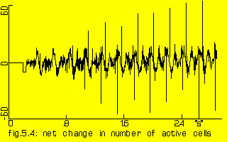
The net change in number of active ‘cells’ of the model of 1000 cells when the outer shell was activated every 113 steps (=226 ‘ms’). This lasted 85 steps (=170 ‘ms’).
Horizontal axis: simulated time since start of persistent activity
Vertical axis: number of cells.

In order to test the reaction of the block of cells to short disturbances the shell was made active during 10 steps at time step 1400, 1889 and 2378. The total activity exhibited the same pattern as in par. 3.3. The three disturbances caused three very large sharp peaks in the plot of active cells, but soon the normal pattern was restored.

The net change in number of active ‘cells’ of the model of 1000 cells when the outer shell was activated with three pulses, each lasting 85 steps (=170 ‘ms’).
Horizontal axis: simulated time since start of persistent activity
Vertical axis: number of cells.

From theoretical studies (Winfree 1980) and experimental work (Jongsma 1975) it is known that an aggregate of coupled periodically active elements can beat (much) faster than the isolated elements. To see whether such an influence would play a role in this model, the refractory state rules were changed in such a way, that a not stimulated cell would become active after a period of 1000 steps, i.e. Tm = 1000. A simulation of the non-pacemaker model during 5100 time steps resulted in a mean period of 114.6 steps for the central cell and a standard deviation of 0.94, whereas in the pacemaker model these figures were 114.8 resp. 0.86 after a simulation run of 6000 steps. In both cases the pattern of activity of the model was stable up to 4000 steps, after which the level of total activity decreased. Although the introduction of the pacemaker ability to all cells did not influence the behaviour of the model, it was maintained in the model.

3.5 lowering the threshold

The model 3,85,12,0.75 was not sufficiently stable after 4000 steps for the same type of signal analysis as used for the recorded signals during ventricular fibrillation. So the threshold D for the transition to the excited and/or active state was lowered from 25 to 15. This model now showed a stable pattern of total activity with very clear double peaks during 6000 steps. The mean period of the central cell was 111.5 with a standard deviation of 0.67.

This threshold is so low that in the X-direction (the strong coupling) one active cell can activate another, which would result in an excitation front in the X-direction. Analysis of the cells 1,5,5 to 10,5,5 however gave no indication of such a front. The reason for this discrepancy is that approximately a quarter of the cells synchronize in one group and a somewhat larger proportion in another group with a phase shift of half a cycle compared to the first group. The rest of the cells are more or less equally distributed through all phases and their membrane potential variations act as noise to the external electrode. This phenomenon of splitting of the population is described more generally by Winfree 1980 (page 117) for a community of simple, connected clocks, where the aggregate rhythm has two peaks per cycle one-half cycle apart on the average. References to examples and additional analytic models are given by him. A “clock” is defined as a periodical device; its period can be influenced by changing the rate of change of its phase. Winfree also describes in the same book (page 128) how this type of behaviour can also originate in a population of “hourglasses”. An “hourglass” being a clock that runs through its cycle only once, this clearly looks like our model of connected cells, as the absence or presence of the pacemaker rhythm of 2000 msec has no influence on the behaviour of the model.

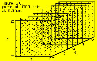
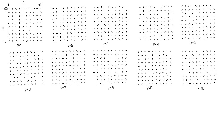
In fig. 5.6 the phases of all 1000 cells from timestep 3120 to 3240 are indicated by the slope of a small linepiece in such a way, that the moment of becoming active of a cell in that period is translated in an angle between 0 and 180 degrees, the vertical lines indicating step 3120 or 3240. The synchronization in two groups is easily seen, just as the many neighbouring cells in opposite phase, as indicated by their phase lines at right angles. The histogram of phases is shown in fig. 5.9.

The shell of cells covering the model was kept quiescent for the above mentioned analysis. In order to study the effect of noisy input from the environment on this small piece of simulated myocard, every time step this shell could be active with a probability of 0.75. The behaviour of the central cell did not change, but the total activity did, although not drastically.

3.6 size considerations

The instabilities of the model are not surprising, if the actual size is considered. An aggregate of 10 by 10 by 10 cells of the dog myocard will have dimensions of circa 1.0 by 0.1 by 0.1 mm. Such a small piece of tissue would stop fibrillation immediately or after several seconds. (Garrey 1914)

Restrictions on available computing time did not make simulations beyond 12 simulated seconds feasible.

Reduction of the size of the model to 512 cells (8�8�8) led to extinction of the activity within 3000 steps.

2.7 Vulnerable period

in cooperation with Annelien Roenhorst

“A striking characteristic of fibrillation is that it can be induced in apparently completely normal hearts by a single stimulus applied during the relatively refractory period, i.e. during the vulnerable period. At that moment some fibers are fully refractory, others are partially refractory and still others have fully repolarized and become normally excitable.” (Cranefield 1975). This phenomenon is also treated by Moe 1941 and Winfree 1983. To find out whether the above mentioned model (without pacemaker activity) possessed a vulnerable period, the ‘environment’ of the model was twice made ‘active’. The threshold D, the duration of activity and the number of timesteps between the ‘pulses’ was varied. If 600 timesteps after the second puls still activity was present, a vulnerable period was concluded. The results are summarized in the next table. Clearly the model contains a vulnerable period; this is a result of the connections between the modelcells and their reactions to stimuli. Until the experiments of A. Roenhorst the existence of this phenomenon in the model was unknown.

stimulus period	stimulus duration in steps
	4	5	6	7	8	9	10
106	15
105	10	10	15		20
104	1	5,10	5,10	10	15		20
103		1	1,5	5,10	10
102				1	5	5,10	10
101						1

table 5.3: Combinations of thresholds, stimulus periods and stimulus durations that caused persistent activity in the {3,88,100,0.75} model

Examples of the reaction of the model to these stimuli is shown in the next figures.

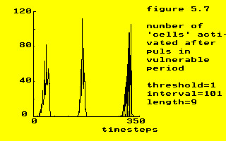
threshold = 1
interval = 101
length = 9

threshold = 20
interval = 105
length = 8

4 Conclusions

The simulations led to a model of a small piece of ventricular tissue, that could maintain a persistent activity during at least 12 simulated seconds. No wavefronts were seen during the very regular activity of the model nor pathways followed by the conducted excitation, in accordance with the results of Ritsema van Eck in his three-dimensional model. ( Ritsema van Eck 1972) In the models of excitable elements in sheets however spiraling wavefronts were reported ( Foy 1974, van Capelle 1980), exactly as Allessie mapped them on the fibrillating atrium.( Allessie 1977)

Foy only states that the wavefront follows a “fairly small, roughly circular path” near the center of his sheet, but Van Capelle and Allessie both indicate a size of approximately 5 mm for the diameter of this circle, around which one or more wavefronts spiral. Winfree (1980) page 310 states in his treatise of an involute spiral wavefront: “the thinness required to justify a two-dimensional description is about the diameter of the troublesome central disk of the involute approximation”. The ventricle is much thicker than this ‘central disk’, so very complicated patterns might develop. Whether the complex periodical pattern of fig. 5.6 can be described as one of Winfree’s three-dimensional rotors has not been investigated.(Winfree 1980)

The splitting of the population of cells with regard to their phases can be seen in the light of the theory of Winfree on networks of simple clocks as mentioned in paragraph 4.5. See Winfree 1980.

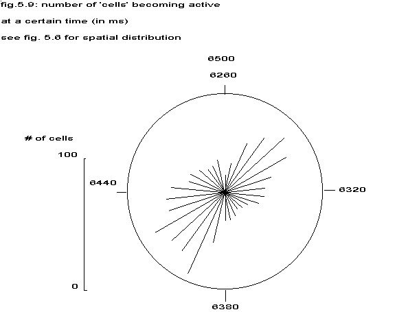
see fig. 5.6 for spatial distribution

Figure 5.9 gives the distribution of cells of the same model results as in fig. 5.6 around the phase circle. The tendency to form two groups in anti-phase is clearly seen. The significance of this splitting into two groups combined with the finding that the repetition rate of the individual cell did not change beyond normal physiological boundaries, will be dealt with in chapter VI, in order to explain the high frequency of ventricular fibrillation.

The fact that the model exhibits persistent, periodical activity as an oscillator, although the constituent elements are not periodically active (at least not in the reported order of magnitude) is by no means a novel finding. The topological model is written in the language of cellular automata and these can behave as an oscillator (Merzenich 1974). More appropriate to the next level of modeling is that stimulations of the model made clear that the model as a whole can be described as a relaxation oscillator, although no attempt has been made to find the set of differential equations that give the same output as the model. However, in chapter VIII formula’s will be given for an oscillator which shows the same overall behaviour as the topological model.

The reader can verify most of the above mentioned results with the program VFMODEL.