DFT and FFT
A Spectral Estimation
B Correlation Functions
C Cross Phase Spectrum
D Autobicoherency Spectrum
E Disappearance of Harmonics from the Spectrum
F ZoomFFT
G Fractals

DFT and FFT

1 Introduction

At the time Jenkins and Watts wrote their book on spectral analysis of signals, an integrated approach using both correlation functions and spectra was possible, as they estimated spectra from the correlation functions. Jenkins 1968 . The introduction of the so-called Fast Fourier Transform (FFT) algorithm by Cooley and Tukey in 1965 Rabiner 1972 , improved 4 years later Singleton 1969 , opened in principle the way to estimate the correlation functions from the Fourier coefficients with a strongly reduced computation time. To get a correlation function directly from a series of N values one needs in general N² multiplications, but via FFT only N(1+²log N) multiplications. If one would store the Fourier coefficients on some magnetic medium, estimation of spectra would only require some additions and divisions. As will be demonstrated in appendix B , naively performing a forward FFT, getting the spectrum and performing a backward FFT will result in a strongly biased estimate of the autocorrelation function. The presented algorithm operates on 2N values, so the total amount of calculations increases to 2N(2+²log N), still considerably less than N² for large N.

The need to handle a big variety of correlation functions and spectra for a large amount of data arose from our research in electrical signals from the heart, recorded in upto 12 simultaneous channels.

Although advanced signal analysis technics segment a series in overlapping pieces – Welch 1967 and Harris 1978 – the method presented in this article sticks to the simple Bartlett procedure of segmenting the series in a number of consecutive blocks of equal length and estimating the spectra from the averaged complex periodograms. In the first place this method was chosen to get unbiased estimates of the correlation functions and in the second place because of ease of computation and the fact, that a comparison between a 4-term Blackman-Harris filter Harris 1978 and the Bartlett smoothing procedure Jenkins 1968 did not show a big difference for our signals.

The next two paragraphs of this chapter will give the theoretical background for the procedure in paragraph 5, which differs from the procedure in a textbook like that of Oppenheim and Schafer Oppenheim 1975 , that after segmenting the input in K blocks of length M and augmenting these blocks with M zeroes Champeney 1973 , the correlation functions are estimated over K-1 blocks instead of K blocks, cross correlation functions may be computed, the estimates of the correlation coefficients will be found in the negative array elements and the spectral components only in the even elements.

2 Notations

 x(n), y(n)    input series
 N=K·M         length of x(n) and y(n)
 M             length of one block
 L=2M          length of one block, augmented with zeroes
 x((m)){N}     periodical series with period N,
               i.e. x(m+K·N) = x(m-K·N) = x(m), K=0,1,2,....
                     N-1         kn 
 DFT           X(k) = 
 x(n)·W{N} 
                     n=0                                   -i(2
/N)
                         N-1         -kn           W{N} = e
 inverse DFT   x(n) = 1/N 
 X(k)·W{N} 
                         k=0 
 c{xy}(m)      estimator of the m-th correlation coefficient, 0<=m<=M
 R{xy}(k)      mean estimator of real part of spectrum
 Q{xy}(k)      mean estimator of imaginary part of spectrum
 C{xy}(k)      mean energy spectrum

3 Correlation

In general the arguments of Oppenheim & Schafer Oppenheim 1975 will be followed with a few slight but important changes. The starting point is the definition of the cross correlation function by Champeney Champeney 1973 :

                       +
                  +

 c{fg}(x) = f(x)*g(x) = 
 f*(x1)g(x1+x)dx1 = 
 f*(x1-x)g(x1)dx1
                       -
                  -

and his extension of the Wiener-Khintchine theorem:

 FT(f(x)*g(x)) = F*(y)G*(y)

where F*(y) stands for the complex conjugate of the Fourier transform of f(x). Now for discrete functions the estimate of the cross correlation will be:

             N-|m|-1               |1-N<=m<=N-1
 c{xy}(m) = 1/N 
 x*(n)y(n+m)      |x(n)=0   |for n<0 and n>N
               n=0                 |y(n)=0   |

As the function is split into K consecutive blocks of length M and the considered functions are real, this expression may be written as:

                M-1            2M-1                KM-1
 c{xy}(m) = 1/N( 
 x(n)y(n+m) + 
 x(n)y(n+m) + ... + 
 x(n)y(n+m) )
                n=0             n=M               n=(K-1)M

using the supposition that x(n) and y(n) are equal to 0 outside the interval 0<=n<=N-1. Considering now the situation that m is not negative, after suitable substitution, this expression may be written as:

                K   M-1
 c{xy}(m) = 1/N 
   
 x(n + (j-1)M) y(n + (j-1)M + m)
               j=1 n=0

For simplification will be defined:

          M-1
 v{j}(m) = 
 x(n + (j-1)M) y(n + (j-1)M + m)
          n=0
                    K
 so: c{xy}(m) = 1/N 
 v{j}(m), with 0<=m<=M-1.
                   j=1

Now keeping in mind that DFT of the blocks means in principle that the considered blocks are supposed to be periodical, the estimation of the correlation function just by DFT implies a circular correlation, where the end of a function is correlated with the beginning of that function, which is not the intention. This is expressed in formula form as:

          M-1
 v{j}(m) = 
 x((n + (j-1)M)){(j-1)M} y((n + (j-1)M + m)){(j-1)M}
          n=0

Define:

 x{j}(n) = x(n+(j-1)M)    0<=n<=M-1
           0              M<=n<=L-1
 y{j}(n) = y(n+(j-1)M)    0<=n<=L-1                            (1)
 where L=2M.

Now the circular correlation:

          M-1
 v{j}(m) = 
 x{j}((n)){L} y{j}((n+m){L}
          n=0

yields for 0<=m<=M-1 the wanted, correct estimates of the correlation coefficients. With X{j}(k) and Y{j}(k) as the L-point DFT’s of x{j}(n) and y{j}(n), the above expression may be written as:

                    L-1           km
 v{j}((-m)){L} = 1/L 
 V{j}(k)W{j}      0<=m<=M-1
                    k=0

where V{j}(k) = X{j}(k)Y{j}*(k), because in general holds:

   _
 FT (F*(y)) =f*(-x)

and as the correlation function is real:

 V{j}*((-m)){L} = V{j}((-m)){L}.
               K-1
 Define: V(k) = 
 V{j}(k)     k=0,1,...,L-1                       (2)
               j=1
                                L-1      i(2p/L)km
 so: c{xy}(m) = 1/N v((-m)){L} = 
 V(k)e                          (3)
                                k=0

Expression (2) differs from expression 11.77 of Oppenheim and Schafer Oppenheim 1975 in the upper limit of the summation. These authors use K as upper limit, which means that the last x-block is correlated with a non-existing y-block. Expression (3) differs from expression 11.78 of Oppenheim and Schafer in the circular description of v; as FFT procedures operate on complex functions, the estimates of the correlation coefficients c(0), c(1), c(2), etc. will be found in v(0), v(-1), v(-2), etc. See appendix B for more explanation. Furthermore the present treatment extends their procedure for auto correlation to cross correlation. If c{xy}(-1), c{xy}(-2) etc. are to be estimated, repeat the above procedure with x(n) and y(n) interchanged. To estimate an auto correlation obviously take x(n)=y(n). Definition (1) may be written as:

 y{j}(n) = y{j}(n')+y{j+1}(n''-M),    n'=0,1,...,M-1;    n''=M,M+1,...,L-1

This means a shift of half a period (M=L/2), so the DFT of y is:

                          k
 Y{j}(k) = Y'{j}(k) + (-1) Y'{j+1}(k)      k=0,1,2,...,L-1

where Y'{j} stands for the DFT of y{j}(n) defined in the same way as x{j}(n) above. All blocks are thus expanded with zeroes to their double length and V{j}(k) is now defined as:

                                   k
 V{j}(k) = X{j}(k)(Y'{j}*(k) + (-1) Y'{j+1}(k)).

A consequence of this method is, that no estimate of correlation coefficients is possible when M=N. The easiest way to scale the calculated inverse Fourier coefficients to correlation coefficients, is to divide all coefficients by c{xx}(0)c{yy}(0).

4 Spectra

The estimation of all kinds of spectra is now complicated by the fact that the blocks are expanded with zeroes to their double length. This expansion of a block x(n) with length M with M zeroes can be considered as multiplication of a block z(n) with length L=2M with the function:

 y(n) = 1    0&ltn&ltM
      = 0    M<=n&ltL

This means in the Fourier domain a convolution of Z(k) with Y(k), where Z and Y represent the Fourier transforms of z and y. Now holds:

       L-1        kn M-1 -i(2
/L)kn    -i(
k/2) sin(
k/2)
 Y(k) = 
 y(n)W{L}  = 
 e          = e sin(
k/L)                 (4)
       n=0           n=0 
 k=1,2,...,L-1 and Y(0)=M, provided M is even.

For the sake of simplicity Z’ is defined as:

         c     m=j
 Z'(m) = c*    m=L-j                                             (5)
         0     all other values of m

where 0<=j<=M-1 and c is a complex value representing the sine and cosine components of one frequency in j.
The Fourier transform of x(n) may now be written as:

 X(k) = (Z'(j)Y((k-j)){L} + Z'(L-j)Y((k+j)){L})/L

The following situations can occur, keeping in mind the fact that according to (4) Y(k)=0 for k=2,4,6,…:

j is even
1. k=j X(k)=(Z'(j)Y(0) + Z'(L-j)Y(2j))/L = ½Z'(j)
2. k=L-j X(k)=(Z'(j)Y(L-2j) + Z'(L-j)Y(0))/L = ½Z'(L-j)
3. k is even, but unequal to j or L-j: both Y((k-j)){L} and Y((k+j)){L} have even parameters, so they equal zero, see (5).
4. k is odd: X(k) has some arbitrary value
j is odd: the same conlusions will be drawn as in the case j is even.

The simplification of (5) was introduced to facilitate the explanation, but as every signal may be thought of as being built by a summation of independent sines and cosines, the conclusion is that X(0), X(2), X(4), etc. contain the Fourier coefficients of x(n), whereas X(1), X(3), X(5), etc. contain arbitrary values not representing spectral components. Removal of the odd elements of X results in M coefficients in X, as should be.

5 Procedure

The theory of this article will now be illustrated by an example of estimation of the auto correlation function and the power spectrum of a cosine. In the course of the illustration the procedure steps will be indicated by roman numerals.

I. Form the input, consisting of K consecutive blocks, each with M equally spaced samples; M must be even.

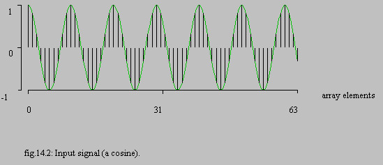
In fig. 14.2 a sampled cosine has been sketched with 2 blocks of 32 samples each. Straight forward Fourier transformation of the whole array of 64 samples yields the power spectrum of fig. 14.3.

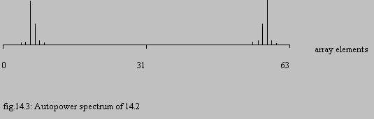
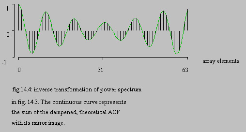
The inverse Fourier transformation of the power spectrum does not result in the auto correlation function, but in a mixture of the theoretical auto correlation (i.e. the same cosine function as the input) linearly decreased to zero at the end of the array, with its mirror image. See fig. 14.4.

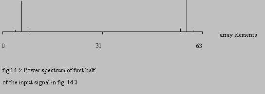
In fig. 14.5 the power spectrum of the first block has been sketched, with its inverse transform in fig. 14.6.

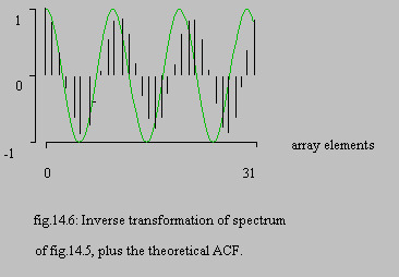
Added to the last figure is the theoretical auto correlation function, which clearly shows the apparent change in period, caused by the “folding back” of the negative part of the auto correlation function, as indicated above in fig. 14.4. If the form of the auto correlation function is unknown, the “unfolding” from the mixture is not possible.

Augment each block with M zeroes and calculate the Discrete Fourier Transform of the blocks.

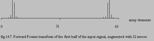
Fig. 14.7 shows the power spectrum of the first block, augmented with zeroes. Comparison with fig. 14.3 and fig. 14.5 clearly indicates that the even elements in fig. 14.7 contain the power spectrum and that the odd elements should be neglected.

Determine the sequences: K-1 k V(k) = X{j}(k)(Y{j}*(k) + (-1) Y{j+1}*(k)) j=1 k=0,1,2,…,L-1 K-1 k B(k) = Y{j}(k)(X{j}*(k) + (-1) X{j+1}*(k)) j=1 where X{j} and Y{j} stands for the DFT of the j-th input block of the inputs x and y resp.; K is the number of blocks, L=2M the length of the block.
Calculate the inverse DFT of V(k) and B(k).
Create the sequence: _ v(L-k+1) k=1,2,3,…,M-1 v=FT (V) c{xy}(k) = v(0) k=0 _ b(L+k+1) k=-1,-2,-3,…,1-M b=FT (B) After division of c{xy} by c{xx}(0)c{yy}(0) the array c contains the cross correlation coefficients. For estimation of the auto correlation function the steps involving B or b should be ignored and y should be substituted by x.

The sequence v after inverse DFT is shown in fig. 14.8 in order to illustrate the position of the auto correlation function in this sequence. The left half of v exhibits the same phenomenon as fig. 14.4 and fig. 14.6.

In order to estimate all types of spectra use only the even elements of the DFT’s of the blocks as calculated in II).

6 Acknowledgements

The research for this article and the implementation of the necessary programs on the Cyber 73/28 of the Rijksuniversiteit Utrecht was made possible by grant 74.101 of the Nederlandse Hartstichting (Netherlands Heart Foundation) and the hard work of Jan Klein Douwel.

A. Spectral estimation

1 Introduction

The theoretical aspects of Discrete Fourier Transformation (DFT) are treated in DFT and FFT .
The method to improve the accuracy of the spectral estimators by averaging over K blocks was originally given by Bartlett. Jenkins 1968 This procedure is equivalent to a spectral window:

            (sin
fM)²
   W(f) = M ( 
fM  )
   or "lag window"
                |u|
            1 - ---     |u| <= M
   w(u) =        M
           
            0           |u| > M

2 First order spectra

In the next formula’s the notation of DFT and FFT is used; because of the Bartlett averaging v=3K.

                                             K
   cospectra     R{xy}(k) = real part of 1/K 
 X{j}(k)Y{j}(k)
                                            j=1
                                                  K
                 Q{xy}(k) = imaginary part of 1/K 
 X{j}(k)Y{j}(k)
                                                 j=1
   powerspectra  C{xy}(k) = 
(R²{xy}(k) + Q²{xy}(k))
                 confidence interval: C(k)/G(k) follows a chi-square (v)
                   distribution.
   phasespectra  F{xy}(k) = arctan (Q{xy}(k)/R{xy}(k))
                 1-
 confidence interval:
                 arcsin 
(2/(v-2)f{2,v-2}(1-
)·(1-K²{xy}(k))/K²{xy}(k))
                 where f{2,v-2}{1-
) stands for the F-distribution.
   coherencyspectra  K²{xy}(k) = C²{xy}(k) / C{xx}(k)C{yy}(k)
   bandwidth     Barlett averaging: 3/2M.

3 Second order spectra

A bispectrum indicates non-linear relations between periodicities in a signal. The only bispectrum used is the autobicoherency. See appendix D for further explanation.

4 Tapering

Taking a block of finite length M out of a series implicates multiplication of the original series with a rectangular window of length M. I.e. the actual Fourier coefficients of the series are convoluted in the Fourier domain by a sinc-function with considerable side-lobes, causing “frequency leakage”.
In order to reduce these sidelobes one could apply a socalled cosine taper – g{ }(t) – to the block to round the sharp edges of the window. In this case the window becomes:

               ½(1-cos((
/
)(t/M)))     0 <= t/M <= 

   g{
}(t) =   1                        
 < t/M < 1-
, with 0 <= 
 <= ½
               ½(1-cos((
/
)(1-t/M)))   1-
 <= t/M <= 1

Thus the leak of spectral energy to farther away frequencies is reduced, but the discriminative power also reduces with a factor 1/(1- ); furthermore a part of the total power is removed.
Three methods are commonly used for improving spectrum estimation by FFT: tapering (e.g. by a cosine function), simple averaging (Bartlett) or averaging with added zeroes (this study). The last method is the best of these three, Yuen 1979 .

5 Zero offset

In order to prevent the leakage of power from Fourier coefficient 0 (“DC component”) into nearby frequency bands, the mean block amplitude was subtracted from the amplitudes in a block prior to DFT. In this way also a certain trendcorrection in the correlogram was possible.

6 Ergodicity

All confidence intervals given are valid only under the assumption of ergodicity, i.e.: if there is no correlation between successive blocks. One can test the ergodicity with the autocorrelation function.

B. Correlation functions and DFT

In DFT and FFT the mathematical reasons are given for using the right (negative) half of the array of Fourier coefficients after transformation of the power spectrum for estimating the correlation function.
No author writing about Fourier transforms indicates this phenomenon (as far as I know). Maybe the reason is this: a forward Fourier transform uses an exponent with a sign opposite to the sign of the exponent of the backward transform; traditionally the electronics engineers use a positive sign for forward and the mathematicians a negative sign. The algorithms of Cooley & Tukey and of Singleton (see Rabiner 1972 , Singleton 1969 and van der Steen 1978 ) assume the positive sign for the forward transform, whereas all other authors known to me use the negative sign. Consult Jenkins 1968 page 314, Gold 1969 page 161, Box 1970 page 45, Rabiner 1972 page 357, Champeney 1973 page 10, Oppenheim 1975 page 284, Randall 1977 pages 15 & 186 and Bracewell 1978 page 362.
If we define the forward transform with negative sign as:

            _
   F(y) = FT {F(x)}
   then:
     +
   FT {(f(x)} = 1/(2
)F(-y)

and there is a switch between the positive and negative parts. Champeney 1973 , page 20.

C. Cross phase spectrum

1 Cross phase versus cross correlation

In estimating a time lag between two somehow related signals, the averaged cross phase spectrum gives a more accurate estimate than the cross correlation function (CCF).

If we express the time lag between two signals as an angle f at a certain frequency F, than clearly f can only assume N discrete values, where N = sampling-frequency / F.
Averaging over blocks will of course give a more accurate estimate, whereas a dampened correlation function does not give a higher accuracy than the sampling frequency.
A time lag will express itself as a displacement of the highest peak in the CCF away from point 0. On the other hand a displacement in the CCF does not imply a time lag. A time lag will express itself as a linear series of phase differences at relevant frequencies. A non-linear series of phase differences could be accompanied by a displacement in the cross correlation function, but means: NO TIME LAG.

2 Unipolar and bipolar signals

The notation used is the same as in appendix A .
If a unipolar signal f{a} forms a Fourier pair with F{x} and another unipolar signal f{b} = Af{a+t}, then f{b} forms a pair with F{y} = A.exp(itx)F{x}.
Now the bipolar signal f{c} = f{a}-f{b} forms a pair with F{z} = (1-A.exp(itx))F{x}.
Denoting at a certain frequency k F{x}(k)=a+ib, then:
R{xy}(k) = A.(a2+b2)costk
Q{xy}(k) = A.(a2+b2)sintk
and
F{xy}(k) = arctan (sintk/costk) = tk;

R{xz}(k) = (a2+b2)(1-A.costk)
Q{xz}(k) = (a2+b2)(1-A.sintk)
and
F{xz}(k) = arctan ((1-A.sintk)/(1-A.costk)).

Clearly if F{xy}(k) and F{xz}(k) are known, A can be calculated.

D. Autobicoherency

Using the notation of appendix A the autobicoherency function is defined as:

                     K
                     
  X{j}(k)X{j}(n)X'{j}(k+n)         k = 0,1,2,...,M
                    j=1                                  n = 0,1,2,...,M
    Bic{xxx}(k,n) = ____________________________         k+n <= M
                    
(C{xx}(k)C{xx}(n)C{xx}(k+n))        X' complex conjugate

This measure lies between 0 and 1; if Bic = 1, then there exists a complete phase-lock between the frequencies f(k), f(n) and f(k)+f(n). If Bic = 0 there is no phase-lock at all.
With ‘phase-lock’ is meant that the phase difference at the frequencies mentioned is constant, taking into account the frequency differences. E.g. if the phase at f(k) = p, then the phase at f(2k) should be: 2p.
Using a taper of (see appendix A par. 4 ) the measure 3c/K follows a chi- square(2) distribution, where c = 1+615/512· +… if is small; see Huber 1971 .
The Bic as defined above has two disadvantages:

as explained in appendix A a taper has several shortcomings;
in estimating Bic by performing FFT and calculating estimators for the spectra, Bic can be much larger than 1; this is caused by inacuracies in finite length numbers in digital computers if relatively large and small numbers are multiplied and divided by each other, see Dumermuth 1971 .

We decided to “pre-whiten” the Bic, i.e. dividing Bic by its amplitude and never found any Bic larger than 1. Using the reasoning of Huber we choose the number 0.5687 as a 0.001 significance level for the mean of 20 not overlapping blocks without tapering.

E. Disappearance of harmonics from the spectrum

1 Introduction

In this chapter a mathematical explanation will be given of the equidis- tant peaks found in power spectra during ventricular fibrillation. No mathematically rigorous treatment will be given. The derivation of the formula’s used will be found in numerous textbook, e.g.: Champeney 1973 and Bracewell 1978 .

2 Equidistant peaks

Repetititon of a function A(t) ad infinitum at regular intervals t{o} removes all of the Fourier transform except delta functions samples at:
y = n.(2 /t{o}); n = 0, ±1, ±2, ….

This is due to the fact that such a repetition can be considered as a convolution of A(t) with a train of delta functions spaced at an interval of t{o}. In formula:

                    +

     E(t) = A(t) ×  
  
(t-n.t{o})
                   n=-

A convolution in the time domain is equivalent to a multiplication in the Fourier domain, so if a(y) is the Fourier transform of A(t), then the Fourier transform of E(t) will be:

                    +

     e(y) = a(y) .  
  
(y-n.2
/t{o}).2
/t{o}                     (E.1)
                   n=-

3 Nomograms

If the repetition of a function is not strictly regular, the equidistant peaks will broaden; the irregular the repetition, the broader the peaks.
The spectra of trains of delta functions were estimated in the usual way (chapter III, par. 4.4 ). The mean interval of these trains was 16/f (f = sampling frequency), so the spectra contain maximal 8 peaks. The intervals were drawn from a Gaussian distribution with mean 16/f and several standard deviations.
In order to be dimension independent the coefficient of variation ( /µ) is used; circa 95 % of the intervals lie in the range (1 ± 2 /µ).µ.

coefficient of variation /µ	figure	coefficient of variation /µ	figure
0		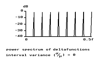0.025
0.05		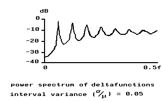0.075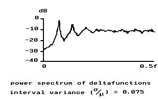
0.094		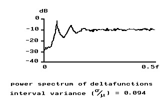0.125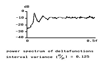
0.156		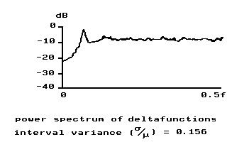0.188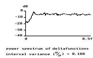
0.25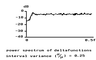

4 Half period shift

Shifting E(t) a distance of ½t{o} is equivalent to convoluting A(t) with:

      +

      
  d(t-t{o}/2-n.t{o})
     n=-

In the Fourier domain this means:

                     +

     e'(y) = a(y) .  
  (-1)n.d(y-n.2
/t{o}).2
/t{o}                 (E.2)
                   n=-

The power spectrum remains unchanged, but the complex spectrum contains alternatively positive and negative peaks (compared to formula E.1). If we now add E(t) with weight (amplitude) factor w to E'(t) with weight factor (1-w) – 0<=w<=1 – then the new spectrum will be the sum of E.1 and E.2 taking the weight factors into account.

                             +

     e(y)+e'(y) = a(y) . w . 
  d(y-n.2
/t{o}).2
/t{o}  +
                            n=-


                                 +

                  a(y) . (1-w) . 
  (-1)n.d(y-n.2
/t{o}).2
/t{o}
                                n=-


                          +

                = a(y) .  
  ((-1)n.(1-w) + w).d(y-n.2
/t{o}).2
/t{o}
                         n=-

The spectral amplitude for odd n is 2w-1 and for even n: 1. If the two signals have the same strength, i.e. w=0.5, then only peaks are found at even n, otherwise more or less small peaks will be found at odd n. The height of the peaks also depends of course on the form of a(y).

5 Conclusion

There are two independent ways peaks (harmonics) can disappear from the spectrum of electrograms during ventricular fibrillation:

an increasingly irregular repetition of the action potentials;
the electrode ‘sees’ two equally strong groups of active cells, firing at the same frequency but with a shift of half a period.

F. ZoomFFT

The result of a normal FFT analysis is distributed in frequency from zero up to the Nyquist frequency (= half the sampling frequency). The frequency resolution is determined by the number of frequency lines up to the Nyquist frequency. Sometimes it is desirable to obtain a considerably finer resolution over a part of the spectrum, so-called “zooming in” on that part Randall 1977 .

Multiplication of a time series with exp(-i2pFt) effectively shifts the frequency origin to frequency F Champeney 1973 . The component at frequency F becomes the new DC component (in general complex). The positive and negative (in relation to F) frequencies are likewise moved by an amount F. This may introduce aliasing in the negative frequency region, as the new Nyquist frequency may lie higher in frequency than the lowest frequency component. After shifting a digital low-pass filter will be required. Note that even if the original signal was real, the modified signal will be complex.

After filtering the signal can be resampled at a lower frequency with a minimum determined by the low-pass filter. In general: to obtain a zoom factor of X, the sample rate should be changed by a factor 2X.

For filtering a physically not realizable zero-phase low-pass filter was constructed Oppenheim 1975 . In the frequency domain a function was constructed consisting of 1’s up to the required filter frequency, followed by 0.5886, 0.1065 and next 0’s up to the original Nyquist frequency. This function was transformed backwards into a time function and then by convolution used as a filter for the shifted signal. The thus obtained new time signal was resampled and the new series was subjected to the normal signal analysis procedures (DFT and FFT ).

G. Fractals

1. L-systems and fractals

This appendix is not intended as a mathematical treatment of fractals. A formal definition of fractals (plus nice pictures) will be found elsewhere Barnsley 1988 and a collection of algorithms and pic- tures in Peitgen 1988 and Lauwerier 1987 .

For the connection between Lindenmayer-systems and fractals see Prusinkiewicz 1989 . Very informally one could say that both L- systems and fractals are defined by a recursive algorithm, contrary to classical geometrical forms, which are defined by a formula. L-systems are excellent tools to describe developing systems ( Rozenberg 1974 and Herman 1975 ). These systems start with an axiom and a finite set of rules, describing how to modify the axiom into a new string and then to modify that string ad infinitum. Adding drawing instructions for a so-called turtle to the rules, these strings can be represented graphically. My program LTURTL.EXE is included in the downloadable file: VFMODEL.ZIP; this file also contains all the fractal rule files mentioned below. LTURTLE.EXE is a Pascal version for the IBM-PC of the Mackintosh C-program of Prusinkiewicz. All his restrictions on its use apply equally to my version; see Prusinkiewicz 1989 .

2. Turtle rules

The reader is free to create new fractals following these instructions:

the Turtle reacts only to:

F	draw a line segment of unit length
f	move a unit length without drawing
+	turn right a specified number of degrees
–	turn left a specified number of degrees
\|	turn around
[	start of a branch
]	end of a branch

3. Fractal rules

An example of plant-like structure (PL3_11B.LTL):

   Derivation length: 30     number of times the rules are applied
   angle factor: 16          Turtle turns 360/16 = 22.5° left or right
   scale factor: 90          100 is full screen
   axiom: F1F1F1
   ignore: +-F               these symbols do not belong to the fractal s.s.
   0 < 0 > 0 --> 1           left of '<' : state of left neigbour
   0 < 0 > 1 --> 1[-F1F1]    between '<' and '>' : state of element
   0 < 1 > 0 --> 1           right of '>' : state of right element
   0 < 1 > 1 --> 1           right of '-->' : new state of element
   1 < 0 > 0 --> 0
   1 < 0 > 1 --> 1F1
   1 < 1 > 0 --> 1
   1 < 1 > 1 --> 0
   * < + > * --> -           '*' : no interaction
   * < - > * --> +

Symbols not mentioned do not change; branches do not belong to the environment of the string they branch of.

The example develops as:

   step  string
    0    F1F1F1
    1    F1F0F1  (rule 8)
    2    F1F1F1F1  (rule 6)
    3    F1F0F0F1  (rule 8)
    4    F1F0F1[-F1F1]F1  (rules 5 & 2)
    5    F1F1F1F1[+F0F1]F1  (rules 6, 4, 9, 8)
      etc.

4. A collection of Prusinkiewicz fractals

Mandelbrot islands and lakes

FRACT4.LTL

A collection of Koch curves

with axiom: F+F+F+F (a square) FRACT5A.LTL 4 steps, * < F > * –> FF+F+F+F+F+F-F FRACT5B.LTL 4 steps, * < F > * –> FF+F+F+F+FF FRACT5C1.LTL 1 step, * < F > * –> FF+F-F+F+FF FRACT5C.LTL 3 steps, * < F > * –> FF+F-F+F+FF FRACT5C4.LTL 4 steps, * < F > * –> FF+F-F+F+FF FRACT5D.LTL 4 steps, * < F > * –> FF+F++F+F FRACT5D5.LTL 5 steps, * < F > * –> FF+F++F+F FRACT5E.LTL 5 steps, * < F > * –> F+FF++F+F FRACT5F.LTL 4 steps, * < F > * –> F+F-F+F+F

A classical dragon curve

FRACT6.LTL

Sierpinsky arrowhead

FRACT8A.LTL

Hexagonal Gosper curve

FRACT8B.LTL

Plants without interaction

PL3_2A.LTL
PL3_2B.LTL
PL3_2C.LTL
PL3_2D.LTL
PL3_2E.LTL

Plants with interaction

PL3_11A.LTL
PL3_11B.LTL
PL3_11C.LTL
PL3_11D.LTL
PL3_11E.LTL

Two kolam patterns

KOLAM_1A.LTL
KOLAM_1C.LTL

Hogeweg plants

No discussion about plant-like fractals is complete without mentioning the pioneering work of Pauline Hogeweg and Ben Hesper Hogeweg 1974 , so included are also my interpretations of two of their figures: HOGE_F2B.LTL and HOGE_F8.LTL.

Barnsley

Figure 3.8.1 of Barnsley 1988 inspired me to:
BARNA2.LTL, 2 derivations
BARNA4.LTL, 4 derivations
BARNA7.LTL, 7 derivations

Figure 3.2.8 inspired me to:
BARNB11.LTL

VF and ECG

To be complete, the ECG-like fractals are:
normal ECG: NORM_ECG.LTL
ventricular fibrillation after tachycardia in VF_ECG.LTL.